Software from CSHL Genome Informatics 2015

I just returned from the Genome Informatics meeting at Cold Spring Harbor. This was, hands down, the best scientific conference I've been to in years. The quality of the talks and posters was excellent, and it was great meeting in person many of the scientists and developers whose tools and software I use on a daily basis. To get a sense of what the meeting was about, 140 characters at a time, you can access all the Tweets sent Oct 28-31 2015 tagged #gi2015 at this link.

Below is a very short list of software that was presented at GI2015. This is only a tiny slice of the tools and methods that were presented at the meeting, and the list is highly biased toward tools that I personally find interesting or useful to my own work (please don't be offended if I omitted your stuff, and feel free to mention it in the comments).

Monocle: Software for analyzing single-cell RNA-seq data
Paper: http://www.nature.com/nbt/journal/v32/n4/full/nbt.2859.html
Software: http://cole-trapnell-lab.github.io/monocle-release/

Kallisto: very fast RNA-seq transcript abundance estimation using pseudoalignment.
Preprint: http://arxiv.org/abs/1505.02710
Software: http://pachterlab.github.io/kallisto/about.html

Sleuth: R package for analyzing & reporting differential expression analysis from transcript abundances estimated with Kallisto.
Preprint: coming soon?
Software: http://pachterlab.github.io/sleuth/about.html
See also: The bear's lair (http://lair.berkeley.edu/): reanalysis of published RNA-seq studies using kallisto+sleuth.

QoRTs: Quality of RNA-Seq Toolset. Toolkit for QC, gene/junction counting, and other miscellaneous downstream processing from RNA-seq alignments.

Software: https://github.com/hartleys/QoRTs

Paper: http://www.ncbi.nlm.nih.gov/pmc/articles/PMC4506620/

JunctionSeq: R package for testing differential junction usage with RNA-seq data.

Software: https://github.com/hartleys/JunctionSeq

Vignette: http://hartleys.github.io/JunctionSeq/doc/JunctionSeq.pdf

HISAT2: RNA-seq alignment against populations of genomes (aligns DNA also).
Software: http://ccb.jhu.edu/software/hisat2/index.shtml

Rail: software for aligning many-sample RNA-seq data, producing alignments, genome coverage bigWigs, and splice junction BED files.
Software: http://rail.bio
Preprint: http://biorxiv.org/content/early/2015/08/11/019067

LobSTR: genotype short tandem repeats from NGS data.
Software: http://melissagymrek.com/lobstr-code/
Paper: http://www.ncbi.nlm.nih.gov/pubmed/22522390

Basset: convolutional neural networks for learning functional/regulatory features of DNA sequence.
Software: https://github.com/davek44/Basset
Preprint: http://biorxiv.org/content/early/2015/10/05/028399

Genotype Query Tools (GQT): fast/efficient individual-level queries of large-scale variation data.
Software: https://github.com/ryanlayer/gqt
Preprint: http://biorxiv.org/content/early/2015/06/05/018259

Centrifuge: a metagenomics classifier.
Software: https://github.com/infphilo/centrifuge
Poster: http://www.ccb.jhu.edu/people/infphilo/data/Centrifuge-poster.pdf

Mash: MinHash-based method for rapidly estimating pairwise distances between genomes or metagenomes.
Software: https://github.com/marbl/Mash
Docs: http://mash.readthedocs.org/en/latest/
Preprint: http://biorxiv.org/content/early/2015/10/26/029827

VCFanno: ultrafast large-sample VCF annotation
Software: https://github.com/brentp/vcfanno

Ginkgo: Interactive analysis and assessment of single-cell copy-number variations
Paper: http://www.nature.com/nmeth/journal/v12/n11/full/nmeth.3578.html
Software: https://github.com/robertaboukhalil/ginkgo

StringTie: RNA-seq transcript assembly+quantification, with or without a reference. See paper for comparison to existing tools.
Software: http://ccb.jhu.edu/software/stringtie/
Source: https://github.com/gpertea/stringtie
Poster: http://ccb.jhu.edu/software/stringtie/cshl2015.pdf
Paper: http://www.nature.com/nbt/journal/v33/n3/full/nbt.3122.html

RNA-seq Data Analysis Course Materials

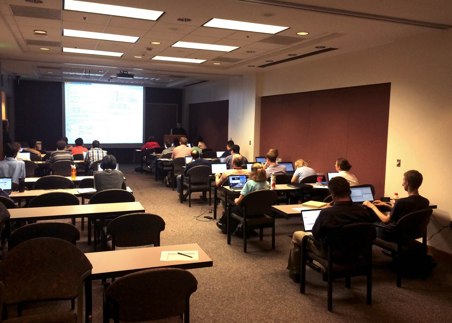
Last week I ran a one-day workshop on RNA-seq data analysis in the UVA Health Sciences Library. I set up an AWS public EC2 image with all the necessary software installed. Participants logged into AWS, launched the image, and we kicked off the morning session with an introduction to the Unix shell (taught by Jessica Bonnie, a biostatistician here in our genomics group, and a fellow Software Carpentry instructor). I followed with a walkthrough of using FastQC for quality assessment, FASTX toolkit for trimming, TopHat for alignment, and featureCounts to summarize gene expression read counts at the gene level. I started the afternoon session started with an introduction to R, followed by a tutorial on analyzing the count data we generated in the first part using DESeq2 in R.

All of the rendered course material is available here. The source code used to generate this material is all on available on GitHub (go read my post on collaborative lesson development, if you haven't already). Much of the introductory Unix lesson material was adapted from the Software Carpentry and Data Carpentry projects.

I wrote a more thorough blog post about how the course went here on the Software Carpentry blog.

I also compiled a PDF of all the course materials, available on Figshare: http://dx.doi.org/10.6084/m9.figshare.1247658.

Introduction to R for Life Scientists: Course Materials

Last week I taught a three-hour introduction to R workshop for life scientists at UVA's Health Sciences Library.

I broke the workshop into three sections:

In the first half hour or so I presented slides giving an overview of R and why R is so awesome. During this session I emphasized reproducible research and gave a demonstration of using knitr + rmarkdown in RStudio to produce a PDF that can easily be recompiled when data updates.

In the second (longest) section, participants had their laptops out with RStudio open coding along with me as I gave an introduction to R data types, functions, getting help, data frames, subsetting, and plotting. Participants were challenged with an exercise requiring them to create a scatter plot using a subset of the built-in mtcars dataset.

We concluded with an analysis of RNA-seq data using the DESeq2 package. We started with a count matrix and a metadata file (the modENCODE pasilla knockout data packaged with DESeq2), imported the data into a DESeqDataSet object, ran the DESeq pipeline, extracted results, and did some basic visualization (MA-plots, PCA, volcano plots, etc). A future day-long course will cover RNA-seq in more detail (intro UNIX, alignment, & quantitation in the morning; intro R, QC, and differential expression analysis in the afternoon).

I wrote the course materials using knitr, rendered using Jekyll, hosted as a GitHub project page. The rendered course materials can be found at the link below, and the source is on GitHub.

Course Materials: Introduction to R for Life Scientists

Slides:



Cheat Sheet:

Using Volcano Plots in R to Visualize Microarray and RNA-seq Results

I've been asked a few times how to make a so-called volcano plot from gene expression results. A volcano plot typically plots some measure of effect on the x-axis (typically the fold change) and the statistical significance on the y-axis (typically the -log10 of the p-value). Genes that are highly dysregulated are farther to the left and right sides, while highly significant changes appear higher on the plot.

I've analyzed some data from GEO (GSE52202) using RNA-seq to study gene expression in motor neurons differentiated from induced pluripotent stem cells (iPSCs) derived from ALS patients carrying the C9ORF72 repeat expansion. I aligned the data, counted with featureCounts, and analyzed with DESeq2. I uploaded the results to this GitHub Gist.

Here's how you can use R to create a simple volcano plot. First, download the results file here and save it as a text file called results.txt.

After reading in the data from GitHub the next section creates a basic volcano plot. A few more lines color the points based on their fold change and statistical significance. Finally, if you have the calibrate package installed, the last line labels a few genes of interest.

Jeff Leek's non-comprehensive list of awesome things other people did in 2013

Jeff Leek, biostats professor at Johns Hopkins and instructor of the Coursera Data Analysis course, recently posted on Simly Statistics this list of awesome things other people accomplished in 2013 in genomics, statistics, and data science.

At risk of sounding too meta, I'll say that this list itself is one of the awesome things that was put together in 2013. You should go browse the entire post for yourself, but I'll highlight a few that I saved to my reading list:

• Yuwen Liu and colleagues published a paper on power for RNA-seq experiments comparing biological replicates and sequencing depth. This paper adds to previous work showing conclusively that adding more replicates is usually better than adding more sequencing depth.
• Thomas Lumley's brief but insightful discussion of statins and the causal Markov property. Lumley also linked to a Labhacks post on a high-quality scrunchable cloth poster print for $25.
• Joe Blitzstein's Data Science course at Harvard, which has an excellent reading list (many are IPython Notebooks, which can be read freely and downloaded to run locally.
• A link to Lior Pachter's blog, which I also regularly read for all things related to RNA-seq and beyond.
• Tuuli Lappalainen's paper on RNA-seq reproducibility. You can also follow Tuuli on Twitter (@tuuliel).
• On the metagenomics front, the metagenomeSeq R package for differential abundance in microbial communities from Mihai Pop's group, and from Curtis Huttenhower's group, a new method for predictive functional profiling of microbial communities using 16S rRNA marker gene sequences.
• Finally, because Jeff's post was about awesome things other people did in 2013, he deliberately omitted some of the awesome things that his own group and others at Johns Hopkins did in 2013. Some of Jeff's contributions that I found most useful in 2013 were several guides, available as GitHub repository READMEs:
• jtleek/rpackages: A guide to developing R packages using devtools, roxygen2, knitr, git, and GitHub.
• jtleek/datasharing: A guide to how to share data with a statistician. This is a great post to send to your collaborators who constantly send you inconsistently coded data without a metadata code book.
• jtleek/reviews: A guide to reviewing academic papers. We've all gotten back terrible, often times useless reviews. Follow the advice here to avoid being one of those awful reviewers we all despise.

This only a sample of what's posted on Jeff's blog. Go read the full post below.

Simply Statistics: A non-comprehensive list of awesome things other people did this year.

Real-time streaming differential RNA-seq analysis with eXpress

RNA-seq has been performed routinely for at least 5+ years, yet there is no consensus on the best methodology for analyzing this data. For example, Eduardo Eyras's group recently posted a pre-print on methods to study splicing from RNA-seq, where this great figure was shown:

This illustrates the problem clearly: ignoring alternative workflows that simply count reads mapping to genes or exons and doing a negative binomial-based test, there are thousands of potential paths through an isoform-resolution RNA-seq analysis.

While the gene/exon-count based approach is simpler and arguably more powerful and well-characterized, there are numerous potential problems with this approach, as outlined in the recent cuffdiff 2 paper:

Reproduced from the cuffdiff2 paper under fair use.

I'm not going to go into the merits of feature-count methods versus transcript deconvolution methods - that discussion is best settled by others.

But if you have the coverage needed for isoform reconstruction, perhaps the most commonly-trodden path through the transcript-resolution differential expression analysis is using TopHat for alignment, Cufflinks for assembly, and Cuffdiff for quantitation and differential expression analysis, as described in this recent protocol.

However, if you've ever used cufflinks with lots of samples or lots of reads, you've noted the exponential increase in computational resources necessary to run the analysis. This problem, as well as the performance of an alternative approach, is illustrated in Fig. 2b in the recent publication about a new tool from Lior Pachter's lab, the un-Google-ably named eXpress, for streaming real-time fragment assignment of RNA-seq data:

Reproduced from the eXpress paper under Fair Use.

I won't attempt to explain here how eXpress works other than to tell you it's EM-based, and to direct you to the paper for a fuller explanation. As you can see from the figure above, the resource requirement with more samples and higher coverage increases linearly, consuming only slightly more RAM than the UNIX wc (word count) command, all the while maintaining accuracy comparable to or slightly better than existing state-of-the-art methods like Cufflinks or RSEM.

So, what's the hold-up? Why isn't everyone using eXpress for differential gene/transcript expression with RNA-seq data? Personal preferences and allegiances aside, part of the reason might be because eXpress's estimated fragment abundances are not true counts, and are not optimally treated as such. Strictly speaking, you can't simply take the transcript abundances you get out of eXpress and throw them into a count-based test like those implemented in edgeR or DESeq, and expect those results to be robust and accurate optimal. What's lacking is a mathematical framework (and a user-friendly R or other software package) for conducting statistical analysis of differential abundance across multiple samples of transcript abundances as estimated by eXpress.

I ran into Lior at the CSHL Genome Informatics meeting this morning, and pressed him on when we might see an R package for statistically analyzing eXpress-estimated isoform abundances, and I was told we would see something within a month. I'm going to hold you to that, Lior, so keep an eye out on Bioconductor and Lior's blog for the much needed and long-awaited statistical framework and R package to do this analysis.

#GI2013 folks, I'll see you at the poster session and reception. And to everyone else, as always, keep calm and sequence on.

De Novo Transcriptome Assembly with Trinity: Protocol and Videos

One of the clearest advantages RNA-seq has over array-based technology for studying gene expression is not needing a reference genome or a pre-existing oligo array. De novo transcriptome assembly allows you to study non-model organisms, cancer cells, or environmental metatranscriptomes. One of the challenges with de novo transcriptome assembly, above and beyond all the challenges associated with genome assembly, is the highly varying abundance (and thus uneven sequencing depth) of different transcripts in a cell.

Several tools have been developed for de novo transcriptome assembly. One of the most widely used is Trinity, developed at the Broad Institute. Trinity is free and open-source, and a recent Nature Protocols article walks through using Trinity for de novo RNA-seq:

Haas, Brian J., et al. "De novo transcript sequence reconstruction from RNA-seq using the Trinity platform for reference generation and analysis." Nature protocols 8.8 (2013): 1494-1512.

In addition, Trinity's creator, Brian Haas, has published four videos on YouTube on de novo transcriptome assembly using Trinity (via RNA-Seq Blog):

Introduction to De Novo RNA-Seq Assembly using Trinity



The General Approach to De novo RNA-Seq Assembly Using De Bruijn Graphs



Trinity - How it works



Strand-specific RNA-Seq is Preferred



Finally, if you're at UVA, we'll be hosting a transcriptome assembly workshop here in November, and registration will be opening soon.

ENCODE ChIP-Seq Significance Tool: Which TFs Regulate my Genes?

I collaborate with several investigators on gene expression projects using both microarray and RNA-seq. After I show a collaborator which genes are dysregulated in a particular condition or tissue, the most common question I get is "what are the transcription factors regulating these genes?"

This isn't the easiest question to answer. You could look at transcription factor binding site position weight matrices like those from TRANSFAC and come up with a list of all factors that potentially hit that site, then perform some kind of enrichment analysis on that. But this involves some programming, and is based solely on sequence motifs, not experimental data.

The ENCODE consortium spent over $100M and generated hundreds of ChIP-seq experiments for different transcription factors and histone modifications across many cell types (if you don't know much about ENCODE, go read the main ENCODE paper, and Sean Eddy's very fair commentary). Regardless of what you might consider "biologically functional", the ENCODE project generated a ton of data, and much of this data is publicly available. But that still doesn't help answer our question, because genes are often bound by multiple TFs, and TFs can bind many regions. We need to perform an enrichment (read: hypergeometric) test to assess an over-representation of experimentally bound transcription factors around our gene targets of interest ("around" also implies that some spatial boundary must be specified). To date, I haven't found a good tool to do this easily.

Raymond Auerbach and Bin Chen in Atul Butte's lab recently developed a resource to address this very common need, called the ENCODE ChIP-Seq Significance Tool.

The paper: Auerbach et al. Relating Genes to Function: Identifying Enriched Transcription Factors using the ENCODE ChIP-Seq Significance Tool. Bioinformatics (2013): 10.1093/bioinformatics/btt316.

The software: ENCODE ChIP-Seq Significance Tool (http://encodeqt.stanford.edu/).

This tool takes a list of "interesting" (significant, dysregulated, etc.) genes as input, and identifies ENCODE transcription factors from this list. Head over to http://encodeqt.stanford.edu/, select the ID type you're using (Ensembl, Symbol, etc), and paste in your list of genes. You can also specify your background set (this has big implications for the significance testing using the hypergeometric distribution). Scroll down some more to tell the tool how far up and downstream you want to look from the transcription start/end site or whole gene, select an ENCODE cell line (or ALL), and hit submit. 

You're then presented with a list of transcription factors that are most likely regulating your input genes (based on overrepresentation of ENCODE ChIP-seq binding sites). Your results can then be saved to CSV or PDF. You can also click on a number in the results table and get a list of genes that are regulated by a particular factor (the numbers do not appear as hyperlinks in my browser, but clicking the number still worked).

At the very bottom of the page, you can load example data that they used in the supplement of their paper, and run through the analysis presented therein. The lead author, Raymond Auerbach, even made a very informative screencast on how to use the tool:

Now, if I could only find a way to do something like this with mouse gene expression data.

Butte Lab: ENCODE ChIP-Seq Significance Tool  (Read the Bioinformatics paper here)

Automated Archival and Visual Analysis of Tweets Mentioning #bog13, Bioinformatics, #rstats, and Others

Automatically Archiving Twitter Results

Ever since Twitter gamed its own API and killed off great services like IFTTT triggers, I've been looking for a way to automatically archive tweets containing certain search terms of interest to me. Twitter's built-in search is limited, and I wanted to archive interesting tweets for future reference and to start playing around with some basic text / trend analysis.

Enter t - the twitter command-line interface. t is a command-line power tool for doing all sorts of powerful Twitter queries using the command line. See t's documentation for examples.

I wrote this script that uses the t utility to search Twitter separately for a set of specified keywords, and append those results to a file. The comments at the end of the script also show you how to commit changes to a git repository, push to GitHub, and automate the entire process to run twice a day with a cron job. Here's the code as of May 14, 2013:



That script, and results for searching for "bioinformatics", "metagenomics", "#rstats", "rna-seq", and "#bog13" (the Biology of Genomes 2013 meeting) are all in the GitHub repository below. (Please note that these results update dynamically, and searching Twitter at any point could possibly result in returning some unsavory Tweets.)

https://github.com/stephenturner/twitterchive

Analyzing Tweets using R

You'll also find an analysis subdirectory, containing some R code to produce barplots showing the number of tweets per day over the last month, frequency of tweets by hour of the day, the most used hashtags within a search, the most prolific tweeters, and a ubiquitous word cloud. Much of this code is inspired by Neil Saunders's analysis of Tweets from ISMB 2012. Here's the code as of May 14, 2013:



Also in that analysis directory you'll see periodically updated plots for the results of the queries above.

Analyzing Tweets mentioning "bioinformatics"

Using the bioinformatics query, here are the number of tweets per day over the last month:

Here is the frequency of "bioinformatics" tweets by hour:

Here are the most used hashtags (other than #bioinformatics):

Here are the most prolific bioinformatics Tweeps:

Here's a wordcloud for all the bioinformatics Tweets since March:

Analyzing Tweets mentioning "#bog13"

The 2013 CSHL Biology of Genomes Meeting took place May 7-11, 2013. I searched and archived Tweets mentioning #bog13 from May 1 through May 14 using this script. You'll notice in the code above that I'm no longer archiving this hashtag. I probably need a better way to temporarily add keywords to the search, but I haven't gotten there yet.

Here are the number of Tweets per day during that period. Tweets clearly peaked a couple days into the meeting, with follow-up commentary trailing off quickly after the meeting ended.

Here is the frequency frequency of Tweets by hour, clearly bimodal:

Top hashtags (other than #bog13). Interestingly #bog14 was the most highly used hashtag, so I'm guessing lots of folks are looking forward to next years' meeting. Also, #ashg12 got lots of mentions, presumably because someone presented updated work from last years' ASHG meeting.

Here were the most prolific Tweeps - many of the usual suspects here, as well as a few new ones (new to me at least):

And finally, the requisite wordcloud:

More analysis

If you look in the analysis directory of the repo you'll find plots like these for other keywords (#rstats, metagenomics, rna-seq, and others to come). I would also like to do some sentiment analysis as Neil did in the ISMB post referenced above, but the sentiment package has since been removed from CRAN. I hear there are other packages for polarity analysis, but I haven't yet figured out how to use them. I've given you the code to do the mundane stuff (parsing the fixed-width files from t, for starters). I'd love to see someone take a stab at some further text mining / polarity / sentiment analysis!

twitterchive - archive and analyze results from a Twitter search

Scotty, We Need More Power! Power, Sample Size, and Coverage Estimation for RNA-Seq

Two of the most common questions at the beginning of an RNA-seq experiments are "how many reads do I need?" and "how many replicates do I need?". This paper describes a web application for designing RNA-seq applications that calculates an appropriate sample size and read depth to satisfy user-defined criteria such as cost, maximum number of reads or replicates attainable, etc. The power and sample size estimations are based on a t-test, which the authors claim, performs no worse than the negative binomial models implemented by popular RNA-seq methods such as DESeq, when there are three or more replicates present. Empirical distributions are taken from either (1) pilot data that the user can upload, or (2) built in publicly available data. The authors find that there is substantial heterogeneity between experiments (technical variation is larger than biological variation in many cases), and that power and sample size estimation will be more accurate when the user provides their own pilot data.

My only complaint, for all the reasons expressed in my previous blog post about why you shouldn't host things like this exclusively on your lab website, is that the code to run this analysis doesn't appear to be available to save, study, modify, maintain, or archive. When lead author Michele Busby leaves Gabor Marth's lab, hopefully the app doesn't fall into the graveyard of computational biology web apps.  Update 2/7/13: Michele Busby created a public Github repository for the Scotty code: https://github.com/mbusby/Scotty

tl;dr? There's a new web app that does power, sample size, and coverage calculations for RNA-seq, but it only works well if the pilot or public data you give it closely matches the actual data you'll collect. 

Paper: Busby, et al. "Scotty: A Web Tool For Designing RNA-Seq Experiments to Measure Differential Gene Expression." Bioinformatics (2013): 10.1093/bioinformatics/btt015.

Web app: http://euler.bc.edu/marthlab/scotty/scotty.php

Source code: https://github.com/mbusby/Scotty

Differential Isoform Expression With RNA-Seq: Are We Really There Yet?

In case you missed it, a new paper was published in Nature Biotechnology on a method for detecting isoform-level differential expression with RNA-seq Data:

Trapnell, Cole, et al. "Differential analysis of gene regulation at transcript resolution with RNA-seq." Nature Biotechnology (2012).

THE PROBLEM

RNA-seq enables transcript-level resolution of gene expression, but there is no proven methodology for simultaneously accounting for biological variability across replicates and uncertainty in mapping fragments to isoforms. One of the most commonly used workflows is to map reads with a tool like Tophat or STAR, use a tool like HTSeq to count the number of reads overlapping a gene, then use a negative-binomial count-based approach such as edgeR or DESeq to assess differential expression at the gene level.  

Figure 1 in the paper illustrates the problem with existing approaches, which only count the number of fragments originating from either the entire gene or constitutive exons only. 

Excerpt from figure 1 from the Cuffdiff 2 paper.

In the top row, a change in gene expression is undetectable by counting reads mapping to any exon, and is underestimated if counting only constitutive exons. In the middle row, an apparent change would be detected, but in the wrong direction if using a count-based method alone rather than accounting for which transcript a read comes from and how long that transcript is. How often situations like the middle row happen in reality, that's anyone's guess.

THE PROPOSED SOLUTION

The method presented in this paper, popularized by the cuffdiff method in the Cufflinks software package, claims to address both of these problems simultaneously by modeling variability in the number of fragments generated by each transcript across biological replicates using a beta negative binomial mixture distribution that accounts for both sources of variability in a transcript's measured expression level. This so-called transcript deconvolution is not computationally trivial, and incredibly difficult to explain, but failure to account for the uncertainty (measurement error) from which transcript a fragment originates from can result in a high false-positive rate, especially when there is significant differential regulation of isoforms. Compared to existing methods, the procedure described claims equivalent sensitivity with a much lower false-positive rate when there is substantial isoform-level variability in gene expression between conditions. 

ALTERNATIVE WORKFLOWS

Importantly, the manuscript also addresses and points out weaknesses several undocumented "alternative" workflows that are discussed often on forums like SEQanswers and anecdotally at meetings. These alternative workflows are variations on a theme: combining transcript-level fragment count estimates (like estimates from Cufflinks, eXpress, or RSEM mapping to a transcriptome), with downstream count-based analysis tools like edgeR/DESeq (both R/Bioconductor packages). This paper points out that none of these tools were meant to be used this way, and doing so violates assumptions of underlying statistics used by  both procedures. However, the authors concede that the variance modeling strategies of edgeR and DESeq are robust, and thus assessed the performance of these "alternative" workflows. The results of those experiments show that the algorithm presented in this paper, cuffdiff 2, outperforms other alternative hybrid Cufflinks/RSEM + edgeR/DESeq workflows [see supplementary figure 77 (yes, 77!]).

REPRODUCIBILITY ISSUES

In theory (and in the simulation studies presented here, see further comments below), the methodology presented here seems to outperform any other competing workflow. So why isn't everyone using it, and why is there so much grumbling about it on forums and at meetings? For many (myself included), the biggest issue is one of reproducibility. There are many discussions about cufflinks/cuffdiff providing drastically different results from one version to the next (see here, here, here, here, and here, for a start). The core I run operates in a production environment where everything I do must be absolutely transparent and reproducible. Reporting drastically different results to my collaborators whenever I update the tools I'm using is very alarming to a biologist, and reduces their confidence in the service I provide and the tools I use. 

Furthermore, a recent methods paper recently compared their tool, DEXSeq, to several different versions of cuffdiff. Here, the authors performed two comparisons: a "proper" comparison, where replicates of treatments (T1-T3) were compared to replicates of controls (C1-C4), and a "mock" comparison, where controls (e.g. C1+C3) were compared to other controls (C2+C4). The most haunting result is shown below, where the "proper" comparison finds relatively few differentially expressed genes, while the "mock" comparison of controls versus other controls finds many, many more differentially expressed genes, and an increasing number with newer versions of cufflinks:

Table S1 from the DEXSeq paper.

This comparison predates the release of Cuffdiff 2, so perhaps this alarming trend ceases with the newer release of Cufflinks. However, it is worth noting that these data shown here are from a real dataset, where all the comparisons in the new Cuffdiff 2 paper were done with simulations. Having done some method development myself, I realize how easy it is to construct a simulation scenario to support nearly any claim you'd like to make.

FINAL THOUGHTS

Most RNA-seq folks would say that the field has a good handle on differential expression at the gene level, while differential expression at isoform-level resolution is still under development. I would tend to agree with this statement, but if cases as presented in Figure 1 of this paper are biologically important and widespread (they very well may be), then perhaps we have some re-thinking to do, even with what we thought were "simple" analyses at the gene level. 

What's your workflow for RNA-seq analysis? Discuss.

STAR: ultrafast universal RNA-seq aligner

There's a new kid on the block for RNA-seq alignment.

Dobin, Alexander, et al. "STAR: ultrafast universal RNA-seq aligner." Bioinformatics (2012).

Aligning RNA-seq data is challenging because reads can overlap splice junctions. Many other RNA-seq alignment algorithms (e.g. Tophat) are built on top of DNA sequence aligners. STAR (Spliced Transcripts Alignment to a Reference) is a standalone RNA-seq alignment algorithm that uses uncompressed suffix arrays and a mapping algorithm similar to those used in large-scale genome alignment tools to align RNA-seq reads to a genomic reference. STAR is over 50 times faster than any other previously published RNA-seq aligner, and outperforms other aligners in both sensitivity and specificity using both simulated and real (replicated) RNA-seq data.

The notable increase in speed comes at the price of a larger memory requirement. STAR requires ~27GB RAM to align reads to a human genome - a moderate amount, but not atypical on most modern servers. STAR aligns ~45 million paired reads per hour per processor, and scales nearly linearly with the number of processors (without appreciably increasing RAM usage). Notably, the STAR algorithm is also capable of handling longer reads such as those from PacBio and the upcoming Oxford Nanopore technologies. STAR is free and open source software.

Dobin, Alexander, et al. "STAR: ultrafast universal RNA-seq aligner." Bioinformatics (2012).

STAR software on Google Code

(This post adapted from my review on F1000).

DESeq vs edgeR Comparison

Update (Dec 18, 2012): Please see this related post I wrote about differential isoform expression analysis with Cuffdiff 2.

DESeq and edgeR are two methods and R packages for analyzing quantitative readouts (in the form of counts) from high-throughput experiments such as RNA-seq or ChIP-seq. After alignment, reads are assigned to a feature, where each feature represents a target transcript, in the case of RNA-Seq, or a binding region, in the case of ChIP-Seq. An important summary statistic is the count of the number of reads in a feature (for RNA-Seq, this read count is a good approximation of transcript abundance).

Methods used to analyze array-based data assume a normally distributed, continuous response variable. However, response variables for digital methods like RNA-seq and ChIP-seq are discrete counts. Thus, both DESeq and edgeR methods are based on the negative binomial distribution.

I see these two tools often used interchangeably, and I wanted to take a look at how they stack up to one another in terms of performance, ease of use, and speed. This isn't meant to be a comprehensive evaluation or "bake-off" between the two methods. This would require complex simulations, parameter sweeps, and evaluation with multiple well-characterized real RNA-seq datasets. Further, this is only a start - a full evaluation would need to be much more comprehensive.

Here, I used the newest versions of both edgeR and DESeq, using the well-characterized Pasilla dataset, available in the pasilla Bioconductor package. The dataset is from an experiment in Drosophila investigating the effect of RNAi knockdown of the splicing factor, pasilla. I used the GLM functionality of both packages, as recommended by the vignettes, for dealing with a multifactorial experiment (condition: treated vs. untreated; library type: single-end and paired-end).



Both packages provide built-in functions for assessing overall similarity between samples using either PCA (DESeq) or MDS (edgeR), although these methods operate on the same underlying data and could easily be switched.

PCA plot on variance stabilized data from DESeq:

MDS plot from edgeR:

Per gene dispersion estimates from DESeq:

Biological coefficient of variation versus abundance (edgeR):

Now, let's see how many statistically significant (FDR<0.05) results each method returns:



In this simple example, DESeq finds 820 genes significantly differentially expressed at FDR<0.05, while edgeR is finds these 820 and an additional 371. Let's take a look at the detected fold changes from both methods:

Here, if genes were found differentially expressed by edgeR only, they're colored red; if found by both, colored green. What's striking here is that for a handful of genes, DESeq is (1) reporting massive fold changes, and (2) not calling them statistically significant. What's going on here?

It turns out that these genes have extremely low counts (usually one or two counts in only one or two samples). The DESeq vignette goes through the logic of independent filtering, showing that the likelihood of a gene being significantly differentially expressed is related to how strongly it's expressed, and advocates for discarding extremely lowly expressed genes, because differential expression is likely not statistically detectable.

Count-based filtering can be achieved two ways. The DESeq vignette demonstrates how to filter based on quantiles, while I used the filtering method demonstrated in the edgeR vignette - removing genes without at least 2 counts per million in at least two samples. This filtering code is commented out above - uncomment to filter.

After filtering, all of the genes shown above with apparently large fold changes as detected by DESeq are removed prior to filtering, and the fold changes correlate much better between the two methods. edgeR still detects ~50% more differentially expressed genes, and it's unclear to me (1) why this is the case, and (2) if this is necessarily a good thing.

Conclusions:

Unfortunately, I may have oversold the title here - this is such a cursory comparison of the two methods that I would hesitate to draw any conclusions about which method is better than the other. In addition to finding more significantly differentially expressed genes (again, not necessarily a good thing), I can say that edgeR was much faster than DESeq for fitting GLM models, but it took slightly longer to estimate the dispersion. Further without any independent filtering, edgeR gave me moderated fold changes for the extremely lowly expressed genes for which DESeq returned logFCs in the 20-30 range (but these transcripts were so lowly expressed anyway, they should have been filtered out before any evaluation).

If there's one thing that will make me use edgeR over DESeq (until I have time to do a more thorough evaluation), it's the fact that using edgeR seems much more natural than DESeq, especially if you're familiar with the limma package (pretty much the standard for analyzing microarray data and other continuously distributed gene expression data). Setting up the design matrix and specifying contrasts feels natural if you're familiar with using limma. Further, the edgeR user guide weighs in at 67 pages, filled with many case studies that will help you in putting together a design matrix for nearly any experimental design: paired designs, time courses, batch effects, interactions, etc. The DESeq documentation is still fantastic, but could benefit from a few more case studies / examples.

What do you think? Anyone want to fork my R code and help do this comparison more comprehensively (more examples, simulated data, speed benchmarking)? Is the analysis above fair? What do you find more easy to use, or is ease-of-use (and thus, reproducibility) even important when considering data analysis?

RNA-Seq & ChiP-Seq Data Analysis Course at EBI

I just got this announcement from EMBL-EBI about an RNA-seq/ChIP-seq analysis hands-on course. Find the full details, schedule, and speaker list here.

Title: Advanced RNA-Seq and Chip-Seq Data Analysis Course
Date: May 1-4 2012
Venue: EMBL-EBI, Hinxton, Nr Cambridge, CB10 1SD, UK
Registration Closing Date: March 6 2012 (12:00 midday GMT)

This course is aimed at advanced PhD students and post-doctoral researchers who are applying or planning to apply high throughput sequencing technologies and bioinformatics methods in their research. The aim of this course is to familiarize the participants with advanced data analysis methodologies and provide hands-on training on the latest analytical approaches.

Lectures will give insight into how biological knowledge can be generated from RNA-seq and ChIP-seq experiments and illustrate different ways of analyzing such data Practicals will consist of computer exercises that will enable the participants to apply statistical methods to the analysis of RNA-seq and ChIP-seq data under the guidance of the lecturers and teaching assistants. Familiarity with the technology and biological use cases of high throughput sequencing is required, as is some experience with R/Bioconductor.

The course covers data analysis of RNA-Seq and ChIP-Seq experiments.
Topics will include: alignment, data handling and visualisation, region identification, differential expression, data quality assessment and statistical analysis, using R/Bioconductor.

An example RNA-Seq Quality Control and Analysis Workflow

I found the slides below on the education page from Bioinformatics & Research Computing at the Whitehead Institute. The first set (PDF) gives an overview of the methods and software available for quality assessment of microarray and RNA-seq experiments using the FastX toolkit and FastQC.



The second set (PDF)  gives an example RNA-seq workflow using TopHat, SAMtools, Python/HTseq, and R/DEseq.



If you're doing any RNA-seq work these are both really nice resources to help you get a command-line based analysis workflow up and running (if you're not using Galaxy for RNA-seq).

Guide to RNA-seq Analysis in Galaxy

James Taylor came to UVA last week and gave an excellent talk on how Galaxy enables transparent and reproducible research in genomics. I'm gearing up to take on several projects that involve next-generation sequencing, and I'm considering installing my own Galaxy framework on a local cluster or on the cloud.

If you've used Galaxy in the past you're probably aware that it allows you to share data, workflows, and histories with other users. New to me was the pages section, where an entire analysis is packaged on a single pages, and vetting is crowdsourced to other Galaxy users in the form of comments and voting.

I recently found a page published by Galaxy user Jeremy that serves as a guide to RNA-seq analysis using Galaxy. If you've never done RNA-seq before it's a great place to start. The guide has all the data you need to get started on an experiment where you'll use TopHat/Bowtie to align reads to a reference genome, and Cufflinks to assemble transcripts and quantify differential gene expression, alternative splicing, etc. The dataset is small, so all the analyses start and finish quickly, allowing you to finish the tutorial in just a few hours. The author was kind enough to include links to relevant sections of the TopHat and Cufflinks documentation where it's needed in the tutorial. Hit the link below to get started.

Galaxy Pages: RNA-seq Analysis Exercise