Exploratory data analysis on P/E ratio of Indian Stocks

Price Earnings ratio (P/E) is one of the very popular ratios reported with all stocks.  Very simply this is thought as - Current Market Price / Earning per Share.   An operational definition of Earning per Share would be Total profit divided by # of Shares .  I will redirect interested readers for further reading to

www.investopedia.com/terms/p/price-earningsratio.asp

In this post, I would just like to show, how we can grab P/E data from Web and create some visualizations on it.  My focus right now is Indian stocks and I intend to use the below website

http://www.indiainfoline.com/MarketStatistics/PE-Ratios/

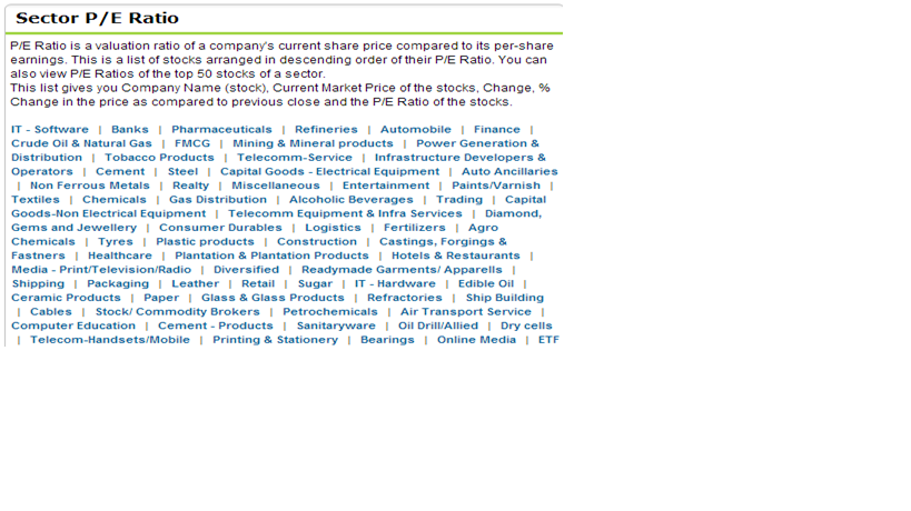
So my first step is gearing up for the data extraction and essentially that is the most non-trivial task.  As shown in the figure below, there is separate pages for each sector and we need to click on individual links , to go to that page and get the P/E ratios.

Here is something , I did outside ‘r’ , creating a csv file with the sector names , using delimiters while importing text and paste special as transpose , here is how my csv file would look.  I would never discourage using multiple tools as this would be required to solve real world issues

So now I can import this in a dataset and read one row at a time and go to necessary URLs , but god have different plans J , it’s not that straightforward

Case 1 :  Single word sector names :

We have sector as ‘Banks’and the sector link is as below

http://www.indiainfoline.com/MarketStatistics/PE-Ratios/Banks-Sector

Again it is a no brainer , we can pick up the base url , append the sector name after a forward slash and then append the string  ‘-Sector’ , this is true for most single word sector names like ‘FMCG’ , ‘Tyres’ , ‘Heathcare’ etc

Case 2:  Multiple words without ‘-‘  , ‘&’ and ‘/’

We have sector as ‘Tobacco Products’ and the sector link is as below

http://www.indiainfoline.com/MarketStatistics/PE-Ratios/Tobacco-Products-Sector

This is also not that difficult apart from adding the ‘-Sector’ we need replace the spaces by a ‘-‘ .

Case 3:  Multiple words with a ‘-‘

We have sector name as ‘IT-Software’, where we have to remove other spaces if exiting. There can be several other cases, but for discussion sake , I will limit myself here

Case 4:  Multiple words with a ‘/‘

We have sector name as ‘Stock/ Commodity Brokers’,  so the “/” needs to be removed

# Reading in dataset

sectorsv1 <- read.csv("C:/Users/user/Desktop/Datasets/sectorsv1.csv")

# Converting to a matrix , this is a practice generally I follow

sectorvm<-as.matrix(sectorsv1)

we can access individual sectors by ,  sectorvm[rowno,colon]

pe<-c()

cname<-c()

cnt<-0

baseurl<-'http://www.indiainfoline.com/MarketStatistics/PE-Ratios/'

sectorvm<-as.matrix(sectorsv1)

for(i in 1:nrow(sectorvm))

{

securl<-sectorvm[i,1]

# Fixed true indicated the string is to matched as is and is not a regular expression

# Substitution of the different cases as we explained , we will point out using gsub instead of sub

# else only the first instance will be replaced

if(length(grep(' ',securl,fixed=TRUE))!=1)

{

securl<-paste(securl,'-Sector', sep="")

}

else

{

securl<-gsub(' ', '-', securl, ignore.case =FALSE, fixed=TRUE)

if(length(grep('---',securl,fixed=TRUE))==1)

{

securl<-gsub(' ---', '-', securl, ignore.case =FALSE, fixed=TRUE)

 }

if(length(grep('&',securl,fixed=TRUE))==1)

{

                securl<-gsub('&', 'and', securl, ignore.case =FALSE, fixed=TRUE)

}

if(length(grep('/',securl,fixed=TRUE))==1)

{

                securl<-gsub('/', '', securl, ignore.case =FALSE, fixed=TRUE)

}

if(length(grep(',',securl,fixed=TRUE))==1)

{

                securl<-gsub(',', '', securl, ignore.case =FALSE, fixed=TRUE)

}

securl<-paste(securl,'-Sector', sep="")

}

fullurl<-paste(baseurl,securl, sep="")

print(fullurl)

if (url.exists(fullurl))

{

petbls<-readHTMLTable(fullurl)

# Exploring the tables we found out relevant information on table 2

# Also the data is getting stored as factor , just doing an as.numeric will not suffice

# we need to do an as.character and then an as.numeric

pe<-c(pe,as.numeric(as.character(petbls[[2]]$PE)))

cname<-c(cname, as.character (petbls[[2]]$Company))

cnt = cnt + 1

}

}

Different functions that we have used are explained as below

readHTMLTables -> Given a url , this function can retrieve the contents of the <Table> tag from html page.  We need to use appropriate no. for the same. Like in this case we have used table no 2.

Grep, Paste, Gsub are normal string functions, grep finds occurrence of a string in another, paste concatenates and gsub does the act of replacing.

As.numeric(as.character()) had a lasting impressing on my mind as an innocuous and intuitive as.numeric would have left me only with the ranks.

url.exists :-> it is a good idea , to check the existence of the url , given we are dynamically forming the URLs.

Now playing with summary statistics:

We use the describe function from psych package

n	mean	sd	median	trimmed	mad	min	max	range	skew	kurtosis	se
1797	59.71	76.92	20.09	46.64	29.79	0	587.5	587.5	2.15	7.25	1.81

hist(pe,col='blue',main='P/E Distribution')

We get the below histogram for the P/E ratio , which shows it is nowhere near a normal distribution , with it’s peakedness and skew as confirmed from the summary statistics as well

We will never the less do a normalty test

shapiro.test(pe)

        Shapiro-Wilk normality test

data:  pe 

W = 0.7496, p-value < 2.2e-16

Basically the null hypothesis is, the values come from a normal distribution and we see the p value to be very insignificant and hence we can easily reject the null.

Drawing a box plot on the P/E ratios

boxplot(pe,col='blue')

Finding the outliers

boxplot.stats(pe)$out

484.33 327.91 587.50

cname[which(pe %in% boxplot.stats(pe)$out)]

[1] "Bajaj Electrical" "BF Utilities"     "Ruchi Infrastr." 

Of course no prize guessing we should stay out of these stocks

So if we summarize this is kind of exploratory data analysis on PE ratio of Indian stocks

·     We saw, we can get content out of url and html tables

·      We added them in a data frame

·       Looked at summary statistics , histogram and did a normality test

·       Plotted a box plot and found the outliers 

Classification using neural net in r

This is mostly for my students and myself for future reference.

Classification is a supervised task , where we need preclassified data and then on new data , I can predict.
Generally we holdout a % from the data available for testing and we call them training and testing data respectively.  So it's like this , if we know which emails are spam , then only using classification we can predict the emails as spam.

I used the dataset http://archive.ics.uci.edu/ml/datasets/seeds# .  The data set has 7 real valued attributes and 1 for predicting .  http://www.jeffheaton.com/2013/06/basic-classification-in-r-neural-networks-and-support-vector-machines/ has influenced many of the writing , probably I am making it more obvious.

The library to be used is library(nnet) , below are the list of commands for your reference

1.       Read from dataset

seeds<-read.csv('seeds.csv',header=T)

2.       Setting training set index ,  210 is the dataset size, 147 is 70 % of that

   seedstrain<- sample(1:210,147)

3.       Setting test set index

   seedstest <- setdiff(1:210,seedstrain)

4.       Normalize the value to be predicted , use that attribute of the dataset , that you want to predict

   ideal <- class.ind(seeds$Class)

5.       Train the model, -8 because you want to leave out the class attribute , the dataset had a total of 8 attributes with the last one as the predicted one

   seedsANN = nnet(seeds[seedstrain,-8], ideal[seedstrain,], size=10, softmax=TRUE)

6.       Predict on training set

   predict(seedsANN, seeds[seedstrain,-8], type="class")

7.       Calculate Classification accuracy

   table(predict(seedsANN, seeds[seedstest,-8], type="class"),seeds[seedstest,]$Class)

Happy Coding !

Opting for shorter movies, be aware u might be cutting the entertainment too!

Hello Friends,

This time I thought to bring in little more spice and thought of focusing on movies.  I don’t know about you but I am a movie buff. Often on a weekend when I am trying to pick up a movie from my movie repository, which spans to some TBs now, I feel little lost.  Apart from a general rating or a perception, the length of the movie plays a role in the choice, simple reason; the movie needs to be cramped between other demanding priorities.

So last Saturday, when I was in between this process, and I was searching for a movie less than 1 hour 30 minutes (There was a hard stop on that) my wife commented but “The short movies are generally not so good”.  I did not pay much heed to that then (Don’t conclude anything from this please), but later on I thought hold on, is that a hypothesis?  Can I do something statistically here?  And here we are. We will talk little bit on correlation, normal distribution etc. I use ‘R’, but it is so simple , we can even use excel sheet do the same.

Correlation:

This is an indicator whose value is between -1 and 1 and it indicates strength of linear relationship between two variables. Leave the jargon, many cases we relate features.  The typical law of physics like speed and displacement may have a perfect correlation, but those are not the point of interest.  However a point of interest may be is there a relation between say

a)      IQ Score of a person and Salary drawn

b)      No. of obese people in an area vis-à-vis no. of fast-food centers in the locality

c)       No. of Facebook friends , with relationship shelf life

d)      No. of hours spent in office and attrition rate for and organization

An underlying technicality, I must point out here is both of the variables should follow a normal distribution.

Normal Distribution:

This is the most common probability distribution function, which is a bell shaped curve, with equal spread in both side of the mean.  Associate to manager alike, you must have heard about normalization and bell curve while you face/do the appraisal.  Most of the random events across disciplines follow normal distribution. The below is an internet image. 

So I picked up movie information and like any one of us picked it up from IMDB (http://www.imdb.com/) and I put it in a structured form like the below, the ones highlighted below may not be required at this point of time, I kept it just for some future work in mind.  The list was prepared manually; I will keep on hunting for some API and all and would keep you posted on the same.

Name	Year of Release	Rating	Duration	Small Desc
Skyfall	2012	8.1	143	Bond's loyalty to M is tested as her past comes back to haunt her. As MI6 comes under attack, 007 must track down and destroy the threat, no matter how personal the cost.

At this point of time I have taken 183 movies.  I have stored it as a csv file.

First thing first, there are various formal ways to test whether it follows a normal distribution, I would just plot histograms and see how this looks like, both the variable seem to follow normal distributions closely.

Below are the commands for a quick reference.  What I just adore about R is it’s simplicity, with just so few commands we are done

film<-read.csv("film.csv",header=T)# Reading the file in a list object

x<-as.matrix(film) # Converting the list to a matrix,  for histogram plotting

y<-as.numeric(x[,3]) # Converting the movie rating to a numeric vector

y<-as.numeric(x[,4]) # Converting the movie duration to a numeric vector

hist(y,col="green",border="black",xlab="Duarion",ylab="mvfreq",main="Mv Duration Distribution",breaks=7)

hist(y,col="blue",border="black",xlab="mvRtng",ylab="mvfreq",main="Mv Rtng Distribution",breaks=9)

cor(y,z) # Calculate Correlation Coefficient between rating and duration

Interestingly the correlation turns out to be .48 in this case, which says there is a positive correlation between this two phenomenon and the correlation is not small.  We can set up a hypothesis “ There is no correlation “ and a level of significance and test the hypothesis. However .48 is a high value and I am sure we would reject the hypothesis that there is no correlation.

So someway or other the rating goes up with the duration of the movie.

I leave it to you for interpretation, but next time you might look at the movie duration for taking a call ! Mr. Directors , it might be a tips for you who knows and may be to me wify is always right. May be all that short is not that sweet.

With that I will call it a day, hope you enjoyed reading. I will be coming on with more such Looking forward to your feedbacks and comments

Venturing in text mining with 'R'

Background:

Hello Friends, hope all of you are doing just great.  I decided to create my footprint in the blog space, it comes from my desire to share few very basic steps of text mining, with all of you.  I am neither a nerd, or statistician or an established data scientist and if you are one of them well, this blog is surely not for you.

I really struggled while I was experimenting with this simple stuff and thought of sharing this with each one of you. I have spent last 6-7 years as a DW & BI professional. I have seen full cycle from data extraction to information delivery, using various tools and technologies and when we talk about advanced analytics it includes advanced data mining/machine learning techniques apart from traditional OLAP.  Predictive analytics will be more relevant with the splurge of data. However I see, lot of my colleagues, across organization finds themselves little awkward, out-of-place while there are talks about dimensionality reduction, Customer Segmentation, Tag Clouding, Anomaly detection.  It is an acknowledged fact that data mining for both structured and unstructured data needs to be much more commoditized in the DWBI Community.  I write to address this gap!  Instead of a bookish bottom-up, I go top-down, with focus on a small yet intuitive task. Again it is not a ‘How to”, so I omit obvious screenshots mostly and try to bring a interactive feel in the narrative. As I said , in case you are an erudite in this field,  venturing further is at your on will and risk, if you are interested about ‘R’ and how this can be used for text mining, I am trying to pen as lucidly as possible, let’s take the plunge together.  So below is the flow, I will describe few terms in my own way and then talk about a simple text mining task.

R:

Well, it’s an open source tool for statistical & visualization tasks.  Formally it is positioned as an environment for Computing and Graphics, it is a successor of S which was developed in Bell labs and it is a part of the GNU.  My inquisitive friends can look at http://cran.r-project.org/ and be further enlightened.  Again informally it is a lightweight convenient tool which is in fact free, and is robust with lot of features.  There are lots of people in different communities, discussion forums and mailing lists .  You don’t need Unix and all, runs smoothly on our own “Windows”. So we can get started with ‘R’ for basic data mining and text mining jobs with any further ado.

Stemming:

I will start with example. Let me put it this way when we are doing a text analysis / mining/ natural language processing or any other kind of task where we deal with words, a basic thing would be looking at distinct words there counts for sure.  So we need to count ‘run’, ‘ran’, ‘running’, ‘runner’ as one word rather than four. So we count the stem of the word rather than the form.

Stop words:

These are frequently used words, which are generally filtered out before a processing task. This is an absolute everyday phenomenon we encounter every day. Stop words can change depending on the nature of the text mining task.

Term Document Matrix:

Don’t scoff at me, if I say text documents are nothing but a very high dimensional vector, and lot of the dimensions are sparsely populated. Texts are high dimensional, simple reason being the words work as dimensions and we know how large than the dimensions can be. Number of dimensions can be as large as number of words in a dictionary. Well there is a popular abstraction of a text document.  We as if start by extracting words one by one from a document and dumping them in a bag.  So we lose the sense of grammar and order of words, but this is still a fairly useful abstraction.  Loosely word and term can be used interchangeably. Only that we might have removed stop words and used stemming, to prune the word list and the final list can be significantly shorter than the original words list.

Coming back to term document matrix in the simplest form, this will have the terms and the frequency against each document. I have taken two very short documents below and then illustrated the term document matrix.  The weights in this case are simple term frequency. However a popular method of weighing is combining the inverse document frequency (IDF) with the same, which takes the rarity of the word also into consideration. I will keep this for subsequent articles may be.

Document1:  Text mining is cool.

Document2:  This is the second text document, with almost no text.

Docs	Almost	cool	document	mining	second	text	The	this	with
1	0	1	0	1	0	1	0	0	0
2	1	0	1	0	1	2	1	1	1

R Installation and getting started:

Well this can be installed from the link I shared earlier.  Follow the version for your OS. I will presume it is for windows and continue, by default setting you would get a shortcut at the desktop.  You click on the same and R gets launched

Text Mining Specific Installation:

You would need to install 2 packages one TM and another Snowball which does not come with default setting.  Go to packages and click on install packages. Select a CRAN Mirror; preferably select one which is geographically closer. Select the packages one by one. Installation happens automatically, we might need to load the packages.

About the task:

You can pick up any task that you want to use the default one as explained in the text mining document “Introduction to the tm Package” or “Text Mining Infrastructure in R”. The second one is a very detailed one, for interested folks, this is definitely must read.  However I thought of making it little different and may be more interesting. I thought of identifying the buzz words/ trends from ‘C’ Levels of IT Offshore based service companies and I thought of choosing N. Chandrasekhar (CEO, TCS) , Francisco D’Souza (CEO, Cognizant ) and S.D.Shibulal ( CEO, Infosys) .  I collected a total of 5 interviews and saved them as 5 text files.  For a broad based trend surely we would need much more documents, but still this can give a decent start. 

Step 1:  Saved the text files in C:<>\Documents\R\win-library\2.15\tm\texts. The path will also depend on the installation options though. I created a folder interviews specific for this and saved the files here. I set the path for tm here

“Intrvw <- system.file("texts", "Interview", package = "tm")”

Step 2: I create a Corpus named “IntrvwC” with these documents

“IntrvwC<-Corpus(DirSource(Intrvw), readerControl = list(reader = readPlain, language = "eng"))”

Step 3: Strip whitespaces from the Corpora

“IntrvwC <- tm_map(IntrvwC, stripWhitespace)”

Step 4: make all the words to lower cases

“IntrvwC <- tm_map(IntrvwC, tolower)”

Step 5: Remove stop-words

“IntrvwC <- tm_map(IntrvwC, removeWords, stopwords("english"))”

Step 6: Remove punctuation

“IntrvwC <- tm_map(IntrvwC, removePunctuation)”

Step 7: Stemming the words

“IntrvwC <- tm_map(IntrvwC, stemDocument)”

Now we are done with our required task and we can look at the document term matrix for this corpora.

The document term matrix

If we just give the name of the document term matrix  at the default R prompt, it will give the below result

A document-term matrix (5 documents, 602 terms)

Non-/sparse entries: 751/2259

Sparsity           : 75%

Maximal term length: 41

Weighting          : term frequency (tf)

Finding frequent terms:

We use the below command

findFreqTerms(dtmIntrvw, 5)

This will identify all the terms that have occurred more than 5 times in the corpora

[1] "business"             "cash"                 "cent"                 "chandrasekaran"       "clients"              "companies"            "company"            

 [8] "customers"            "discretionary"        "don<U+393C><U+3E32>t" "europe"               "financial"            "growth"               "industry"            

[15] "infosys"              "insurance"            "look"                 "margins"              "opportunities"        "quarter"              "services"           

[22] "shibulal"             "spend"                "spending"             "strategic"            "tcs"                  "technology"           "time"

It will be audacious to conclude anything from corpora of five documents. Never the less Europe seems to be in any leadership’s mind none the less.

With that I will sign-off thanks for bearing with me. I would be more than looking forward for your comments. Wish you a happy festive time ahead with your family and friend.