A Little Web Scraping Exercise with XML-Package

Some months ago I posted an example of how to get the links of the contributing blogs on the R-Blogger site. I used readLines() and did some string processing using regular expressions.

With package XML this can be drastically shortened -
see this:

# get blogger urls with XML:
library(RCurl)
library(XML)
script <- getURL("www.r-bloggers.com")
doc <- htmlParse(script)
li <- getNodeSet(doc, "//ul[@class='xoxo blogroll']//a")
urls <- sapply(li, xmlGetAttr, "href")

With only a few lines of code this gives the same result as in the original post! Here I will also process the urls for retrieving links to each blog's start page:

# get ids for those with only 2 slashes (no 3rd in the end):
id <- which(nchar(gsub("[^/]", "", urls )) == 2)
slash_2 <- urls[id]

# find position of 3rd slash occurrence in strings:
slash_stop <- unlist(lapply(str_locate_all(urls, "/"),"[[", 3))
slash_3 <- substring(urls, first = 1, last = slash_stop - 1)

# final result, replace the ones with 2 slashes,
# which are lacking in slash_3:
blogs <- slash_3; blogs[id] <- slash_2

p.s.: Thanks to Vincent Zoonekynd for helping out with the XML syntax.

Applying Same Changes to Multiple Dataframes

How to apply the same changes to several dataframes and
save them to CSV:

# a dataframe
a <- data.frame(x = 1:3, y = 4:6)

# make a list of several dataframes, then apply function (change column names, e.g.):
my.list <- list(a, a)
my.list <- lapply(my.list, function(x) {names(x) <- c("a", "b") ; return(x)})

# save dfs to csv with similar lapply-call:
n <- 1:length(my.list)
lapply(n, function(ni) {
               write.table(file = paste(ni, ".csv", sep = ""), 
               my.list[ni], sep = ";", row.names = F)
               }
       )

Edit:

I'll extend this to a script that reads several files from a directory, applies changes to the files in the same fashion and finally saves files back to the directory (as HERE)

# clean up
rm(list = ls())
setwd(tempdir())
unlink(dir(tempdir()))

# create some files in tempdir:
a <- data.frame(x = 1:3, y = 4:6)
b <- data.frame(x = 10:13, y = 14:15)
write.csv(a, "file1.csv", row.names = F)
write.csv(b, "file2.csv", row.names = F)

# now read all files to list:
mycsv = dir(pattern=".csv")

n <- length(mycsv)
mylist <- vector("list", n)

for(i in 1:n) mylist[[i]] <- read.csv(mycsv[i])

# now change something in all dfs in list:
mylist <- lapply(mylist, function(x) {names(x) <- c("a", "b") ; return(x)})

# then save back dfs:# then save back dfs:
for(i in 1:n) {
   write.csv(file = sub(".csv", "_new.csv", mycsv[i]),
             mylist[i], row.names = F)
}

How to Extract Citation from a Body of Text

Say, you have a text and you want to retrieve the cited names and years of publication. You wouldn't want to this by hand, wouldn't you?

Try the following approach:
(the text sample comes from THIS freely available publication)

library(stringr)

(txt <- readLines("http://dl.dropbox.com/u/68286640/Test_Doc.txt"))
[1] "1  Introduction"                                                                                                                                                                                                                                                                                                                                                                                                                                                                                                                                                                                                                                                                                                                                                                                                                                                                                                                                                                                                                                                                                                                                                                                                                                                                                                                                                                                                                                                             
[2] ""                                                                                                                                                                                                                                                                                                                                                                                                                                                                                                                                                                                                                                                                                                                                                                                                                                                                                                                                                                                                                                                                                                                                                                                                                                                                                                                                                                                                                                                                            
[3] "Climate projections of the Intergovernmental Panel on Climate Change (IPCC) forecast a general increase of seasonal temperatures in the present century across the temperate zone, aggravated by decreasing amounts of summer rainfall in certain regions at lower latitudes (Christensen et al. 2007). These changes imply serious ecological consequences, especially in biome transition zones (Fischlin et al. 2007). Due to their economic importance, as well as their major contribution to supporting, regulating and cultural ecosystem services, predicted changes and shifts in temperate forest ecosystems receive wide public attention. It’s no surprise that dominant forest tree species are frequently modelled in bioclimatic impact studies (e.g., Sykes et al. 1996; Iverson, Prasad 2001; Rehfeldt et al. 2003; Ohlemüller et al. 2006). However, most studies focus on continental-scale effects of climate change, using low resolution climatic and species distribution data. More detailed regional studies focussing on specific endangered regions are also needed (Benito Garzón et al. 2008). Such regional studies have already been prepared for several European regions, including the Swiss Alps (Bolliger et al. 2000), the British Isles (Berry et al. 2002) and the Iberian Peninsula (Benito Garzón et al. 2008)."                                                                                                                    
[4] ""                                                                                                                                                                                                                                                                                                                                                                                                                                                                                                                                                                                                                                                                                                                                                                                                                                                                                                                                                                                                                                                                                                                                                                                                                                                                                                                                                                                                                                                                            
[5] "In this study, we aim to (1) identify the limiting macroclimatic factors and to (2) predict the future boundaries of beech (Fagus sylvatica L.) and sessile oak (Quercus petraea (Mattuschka) Liebl.) forests in a region highly vulnerable to climatic extremes. Both tree species form extensive zonal forests throughout Central Europe and reach their low altitude/low latitude, xeric (Mátyás et al. 2009) distributional limits within the forest-steppe biome transition zone of Hungary. The rise of temperature, and especially summer rainfall deficits expected for the twenty-first century, may strongly affect both species. Nevertheless, regarding the potential future distribution of these important forest tree species along their xeric boundaries in Central Europe, there has been no detailed regional analysis before. Experimental studies and field survey data suggest a strong decline in beech regeneration (Czajkowski et al. 2005; Penuelas et al. 2007; Lenoir et al. 2009) and increased mortality rates following prolonged droughts (Berki et al. 2009). Mass mortality and range retraction are potential consequences, which have been already sporadically observed in field survey studies (Jump et al. 2009; Allen et al. 2010; Mátyás et al. 2009). With the study, we intend to assist in assessing overall risks, locating potentially affected regions and supporting the formulation of appropriate measures and strategies."
[6] ""                                                                                                                                                                                                                                                                                                                                                                                                                                                                                                                                                                                                                                                                                                                                                                                                                                                                                                                                                                                                                                                                                                                                                                                                                                                                                                                                                                                                                                                                            
[7] "Beech and sessile oak forests of Hungary are to a large extent “trailing edge” populations (Hampe and Petit 2005), which should be preferably modelled using specific modelling strategies (Thuiller et al. 2008). Most modelling studies do not differentiate between leading and trailing edges and rely on assumptions and techniques which are intrinsically more appropriate for “leading edge” situations. Being aware of these challenges, we compiled a statistical methodology customized to yield inference on influential variables and providing robust and reliable predictions for climate-dependent populations near their xeric limits. We laid special emphasis on three features in the course of the modelling process: (1) screening of the occurrence data in order to limit modelling to plausible zonal (i.e. macroclimatically determined) occurrences, (2) avoiding pitfalls of statistical pseudoreplication caused by spatial autocorrelation (a problem to which regional distribution modelling studies are particularly prone; Dormann 2007) and (3) simultaneous use of several initial and boundary conditions in an ensemble modelling framework (Araújo et al. 2005; Araújo and New 2007; Beaumont et al. 2007). "                                                                                                                                                                                                                         

# retrieve text inbetween parantheses:
extr1 <- unlist(str_extract_all(txt, pattern = "\\(.*?\\)"))

# keep only those elements which have four digit strings (years):
extr2 <- extr1[grep("[0-9]{4}", extr1)]

# extract partial strings starting with uppercase letter (name)
# and end in a four digit string (year):
(str_extract(extr2, "[A-Z].*[0-9]"))
 [1] "Christensen et al. 2007"                                                              
 [2] "Fischlin et al. 2007"                                                                 
 [3] "Sykes et al. 1996; Iverson, Prasad 2001; Rehfeldt et al. 2003; Ohlemüller et al. 2006"
 [4] "Benito Garzón et al. 2008"                                                            
 [5] "Bolliger et al. 2000"                                                                 
 [6] "Berry et al. 2002"                                                                    
 [7] "Benito Garzón et al. 2008"                                                            
 [8] "Mátyás et al. 2009"                                                                   
 [9] "Czajkowski et al. 2005; Penuelas et al. 2007; Lenoir et al. 2009"                     
[10] "Berki et al. 2009"                                                                    
[11] "Jump et al. 2009; Allen et al. 2010; Mátyás et al. 2009"                              
[12] "Hampe and Petit 2005"                                                                 
[13] "Thuiller et al. 2008"                                                                 
[14] "Dormann 2007"                                                                         
[15] "Araújo et al. 2005; Araújo and New 2007; Beaumont et al. 2007"                        

# as proposed by a commentator -
# do this if you want each citation seperately:
(unlist(str_extract_all(extr2, "[A-Z].*?[0-9]{4}")))
 [1] "Christensen et al. 2007"   "Fischlin et al. 2007"     
 [3] "Sykes et al. 1996"         "Iverson, Prasad 2001"     
 [5] "Rehfeldt et al. 2003"      "Ohlemüller et al. 2006"   
 [7] "Benito Garzón et al. 2008" "Bolliger et al. 2000"     
 [9] "Berry et al. 2002"         "Benito Garzón et al. 2008"
[11] "Mátyás et al. 2009"        "Czajkowski et al. 2005"   
[13] "Penuelas et al. 2007"      "Lenoir et al. 2009"       
[15] "Berki et al. 2009"         "Jump et al. 2009"         
[17] "Allen et al. 2010"         "Mátyás et al. 2009"       
[19] "Hampe and Petit 2005"      "Thuiller et al. 2008"     
[21] "Dormann 2007"              "Araújo et al. 2005"       
[23] "Araújo and New 2007"       "Beaumont et al. 2007"

Classification Trees and Spatial Autocorrelation

I'm currently trying to model species presence / absence data (N = 523) that were collected over a geographic area and are possibly spatially autocorrelated. Samples come from preferential sites (sea level > 1200 m, obligatory presence of permanent waterbodies, etc). My main goal is to infere on environmental factors determining the occurrence rate of several (amphibian) species and to rule out spatial autocorrelation.

Custom Summary Stats as Dataframe or List

On Stackoverflow I found this useful example on how to apply custom statistics on a dataframe and return the results as list or dataframe:

Creating a Stratified Random Sample of a Dataframe

Expanding on a question on Stack Overflow I'll show how to make a stratified random sample of a certain size:

d <- expand.grid(id = 1:35000, stratum = letters[1:10])

p = 0.1

dsample <- data.frame()

system.time(
for(i in levels(d$stratum)) {
  dsub <- subset(d, d$stratum == i)
  B = ceiling(nrow(dsub) * p)
  dsub <- dsub[sample(1:nrow(dsub), B), ]
  dsample <- rbind(dsample, dsub) 
  }
)

# size per stratum in resulting df is 10 % of original size:
table(dsample$stratum)

R-Function to Read Data from Google Docs Spreadsheets

I used this idea posted on Stack Overflow to plug together a function for reading data from Google Docs spreadsheets into R.

Apprentice Piece with Lattice Graphs

Lattice graphs can be quite tedious to learn. I don't use them too often and  when I need them I usually have to dig deep into the archives for details on the parameter details.
The here presented example may serve as a welcome template for the usage of panel functions, panel ordering, for drawing of lattice keys, etc.
You can download the example data HERE.

(Also, check this resource with examples by the lattice-author). 

Testing the Effect of a Factor within each Level of another Factor with R-Package {contrast}

This is a small example of how custom contrasts can easily be applied with the contrast-package. The package-manual has several useful explanations and the below example was actually grabbed from there.
This example can also be applied to a GLM but I choose to use a LM because the coefficients are more easily interpreted.

Transformation of Several Variables in a Dataframe

This is how I transform several columns of a dataframe, i.e., with count-data into binary coded data (this would apply also for any other conversion..).

count1 <- count2 <- count3 <- count4 <- sample(c(rep(0, 10), 1:10))
some <- LETTERS[1:20]  
thing <- letters[1:20]  
mydf <- data.frame(count1, count2, count3, count4, some, thing)

ids <- grep("count", names(mydf))
myfun <- function(x) {ifelse(x > 0, 1, 0)}
mydf[, ids] <- lapply(mydf[, ids], myfun)

p.s.: Let me know if you know of a slicker way.

A Short Example with R-Package osmar..

Following up my last post in which I praised the capabilities of the osmar-package I give a short example...

ps: You can also find this example at GitHub HERE.

osmar - Don't Miss this New R-Geo-Package!

The osmar-package enables you to retrieve all geographic elements of OpenStreetMap via its API.
I.e., you can retrieve a street, river, state-boundary or whatever and use this as a spatial object in R.

It's overwhelming thinking of the endless playground that is opened for R-users by this package!

And, owing to altruistic R-package authors (like the ones of osmar, Thomas Schlesinger and Manuel J. A. Eugster) the oligarch's (ESRI) power evermore crumbles away..

R-Function to Source all Functions from a GitHub Repository

Here's a function that sources all scripts from an arbitrary github-repository. At the moment the function downloads the whole repo and sources functions kept in a folder named "Functions" - this may be adapted for everyones own purpose.

Blog Statistics with StatCounter & R

If you're interested in analysing your blog's statistics this can easily be done with a web-service like StatCounter (free, only registration needed, quite extensive service) and with R.
After implementing the StatCounter script in the html code of a webpage or blog one can download and inspect log-files with R with some short lines of code (like below) and then inspect visitor activity..

Function to Collect Geographic Coordinates for IP-Addresses

I added the function IPtoXY to theBioBucket-Archives which collects geographic coordinates for IP-addresses.

It uses a web-service at http://www.datasciencetoolkit.org// and works with the base R-packages.

# System time to collect coordinates of 100 IP-addresses:
> system.time(sapply(log$IP.Address[1:100], FUN = IPtoXY))
       User      System verstrichen
       0.05        0.02       33.10

Conversion of Several Variables to Factors

..often needed when preparing data for analysis (and usually forgotten until I need it for the next time).
With the below code I convert a set of variables to factors - it could be that there are slicker ways to do it (if you know one let me know!)

> dat <- data.frame(matrix(sample(1:40), 4, 10, dimnames = list(1:4, LETTERS[1:10])))
> str(dat)
'data.frame':   4 obs. of  10 variables:
 $ A: int  5 34 3 15
 $ B: int  28 25 17 24
 $ C: int  2 12 10 32
 $ D: int  16 27 29 14
 $ E: int  40 7 4 31
 $ F: int  22 30 6 18
 $ G: int  33 36 35 38
 $ H: int  19 21 37 8
 $ I: int  20 11 9 26
 $ J: int  39 13 1 23
> 
> id <- which(names(dat)%in%c("A", "F", "I"))
> dat[, id] <- lapply(dat[, id], as.factor)
> str(dat[, id])
'data.frame':   4 obs. of  3 variables:
 $ A: Factor w/ 4 levels "3","5","15","34": 2 4 1 3
 $ F: Factor w/ 4 levels "6","18","22",..: 3 4 1 2
 $ I: Factor w/ 4 levels "9","11","20",..: 3 2 1 4

Some Fun with googleVis - Mapping Blog Visits on Google Map

See stand-alone code to produce this map below.

Default Convenience Functions in R (Rprofile.site)

I keep my blog-reference-functions, snippets, etc., at github and want to source them from there. This can be achieved by utilizing a function (source_https, customized for my purpose HERE). The original function was provided by the R-Blogger Tony Breyal - thanks Tony! As I will use this function quite frequently I just added the function code to my Rprofile.site and now am able to source from github whenever running code from the R-console. This is very handy and I thought it might be worth to share..

Function for Adding Transparency to JPEG (Output = PNG)

..see the function-code HERE.

Animation Newby Excercise with R-Package {animation}

Try this very simple & illustrative example for creating an animation with the animation package:

myfun <- function ( ) {
             n = ani.options("nmax")
             x = sample(1:n)
             y = sample(1:n)

             for (i in 1:n) {
                plot(x[i], y[i], cex = 3, col = 3, pch = 3, , lwd = 2,
                     ylim = c(0, 50),
                     xlim = c(0, 50))
                ani.pause()
                            }
                      }

ani.start()
par(mar = c(3, 3, 1, 0.5), mgp = c(1.5, 0.5, 0), tcl = -0.3)
myfun()
ani.stop()

A Word Cloud with Spatial Meaning

..Some time ago I did a word cloud for representing a Google Scholar search result. Tal Galili pointed me at a post by Drew Conway that expanded on the topic of word clouds lacking spatial meaning. In fact the spatial ordering of words in a word cloud is arbitrary and meaningless..

As I am an ecologist, I soon came to the idea that text could be treated as a multivariate data set - assuming that words can be treated as species and sentences being similar to samples. So, presuming that it makes sense to put sentences and words in a cross-table as I similarly would do with a species / samples matrix, it may also be sensible to analyze such a matrix by ordination-methods for multivariate data, mostly used by ecologist recently. I chose NMDS ordination, as it is robust and quite easy to compute with R-package {vegan}.

Producing Google Map Embeds with R Package googleVis

(1) for producing html code for a Google Map with R-package googleVis do something like:

 

library(googleVis)
df <- data.frame(Address = c("Innsbruck", "Wattens"),
                 Tip = c("My Location 1", "My Location 2"))
mymap <- gvisMap(df, "Address", "Tip", options = list(showTip = TRUE, mapType = "normal",
                 enableScrollWheel = TRUE))
plot(mymap) # preview

(2) then just copy-paste the html to your blog or website after customizing for your purpose..

Retrieve GBIF Species Occurrence Data with Function from dismo Package

..The dismo package is awesome: with some short lines of code you can read & map species distribution data from GBIF (the global biodiversity information facility) easily:

..A Quick Geo-Trick for GoogleMaps in R (using dismo)

... I thought this geocoding-bit might be worth sharing (found HERE when searching the web for dismo-documentation).

..Some More Regex Examples Added to Collection

Find the below examples added to my list of regex-examples HERE.

A Function for Adding up Matrices with Different Dimensions

I couldn't find a function that can handle matrices with different dimensions and thus coded one myself.  It can sum up matrices and also copes with matrices with different dimensions.

Using SyntaxHighlighter and R Brush in Blogger

If you're thinking it is time to give the code examples in your blog a more readable look, you may follow this path and use the SyntaxHighlighter

First thing: check the SyntaxHighlighter Website for the basics.

How to Download and Run Google Docs Script in the R Console

...There is not much to it:

upload a txt file with your script, share it for anyone with the link, then simply run something like the below code. 

ps: When using the code for your own purpose mind to change "https" to "http" and to insert your individual document id.
pss: You could use download.file() in this way for downloading any file from Google Docs..

In Reply to Ben Bolker's Post "Google Scholar (still) sucks"

Replying to Ben Bolker's post Google Scholar (still) sucks:

Ben,

thanks for illustrating the issue in your post!

The main purpose of my function GScholarScraper is to retrieve titles - just because this is the best we can get from Google Scholar. Abstracts are truncated and thus shouldn't be used for meta-analysis. Also titles are truncated, as you said, and there is no way around. Though, this is not as often and severe as with abstracts, i.e.

The CSV is optional, the df with word frequencies and the word cloud are always returned - for any other output one can easily add some appropriate lines to the script.

My opinion:
My function is good for a quick summary and illustration of a query-result.

Tony's function is evidently better if you want to pull all fields of a given query (authors, titles, abstracts,..)

I wonder if people came across ROpenSci? I guess that might be very interesting in this context!

Last remark: Of course, a Google Scholar API would resolve all our problems in this regard..

Best,
Kay

An Image Crossfader Function

Some project offspin, the jpgfader-function (the jpgfader-function in funny use can be viewed HERE):

Add Transparency to JPEG - Yes, We Can!

...Just read in your JPEG and add an alpha channel manually, then assign values for transparency. Of course for printing you need to use a device that accepts alpha.

See how it's done HERE.

R-Function GScholarScraper to Webscrape Google Scholar Search Result

NOTE: You'll find the update HERE and HERE.

NOTE: The script is currently not working because the code of the Google-Scholar site has changed...
I'll see for this as soon as I find some spare time for it!

NOTE: If you try to access GoogleScholar programatically consider this words of caution:
http://stackoverflow.com/questions/7523961/google-scholar-with-matlab/7587994#7587994
...

Based on my previous post on Web Scraping I coded and uploaded the Function "GScholarScraper" HERE for testing!
The function will pull all (!) results, processing pages in chunks of 100 results/titles, and return a file with all titles, links, etc. It will also produce a word cloud using the words in the publication titles.

Please try your own search strings and report errors, etc.!

Build and run properly under:
R version 2.13.0 (2011-04-13) and R version R-2.13.2 (2011-09-30)

Platform: i386-pc-mingw32/i386 (32-bit) locale:
[1] LC_COLLATE=English_United States.1252
[2] LC_CTYPE=English_United States.1252
[3] LC_MONETARY=English_United States.1252
[4] LC_NUMERIC=C
[5] LC_TIME=English_United States.1252

attached base packages:
[1] stats graphics grDevices utils datasets methods base

other attached packages:
[1] stringr_0.5 tm_0.5-6 wordcloud_1.2 Rcpp_0.9.7

loaded via a namespace (and not attached):
[1] plyr_1.5.1 slam_0.1-23

PS: Errors reported lately (see comments) were resolved, the source code was updated..

Next Level Web Scraping

The outcome presented above will not be very useful to most of you - still, this could be a good example for what possibly can be done via webscraping in R.

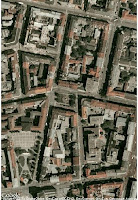
Background: TIRIS is the federal geo-statistical service of North-Tyrol, Austria. One of many great things it provides are historical and recent aerial photographs. These photographs can be addressed via URL's. This is the basis of the script: the URL's are retrieved, some parameters are adjusted, using the customized addresses images are downloaded and animated by saveHTML from the Animation-Package. The outcome (HTML-Animation) enables you to view and skip through aerial photographs of any location in North-Tyrol, from the year 1940 to 2010, and see how the landscape, buildings, etc. have changed...

View the script HERE.

Some Simple but Propably Useful Regex Examples with R-Package stringr...

I found that examples for the use of regex in R are rather rare. Thus, I will provide some examples from my own learning materials - mostly stolen from the help pages, with small but maybe illustrative adaptions. ps: I will extent this list of examples HERE occasionally..

Webscraping Google Scholar & Show Result as Word Cloud Using R

NOTE: Please see the update HERE and HERE!

...When reading Scott Chemberlain's last post about web-scraping I felt it was time to pick up and complete an idea that I was brooding over for some time now:

When a scientist aims out for a new project the first thing to do is to evaluate if other people already have come along to answer the very questions he is about to work on. I.e., I was interested if there has been done any research regarding amphibian diversity at regional/geographical scales correlated to environmental/landscape parameters. Usually I would got to Google-Scholar and search something like - intitle:amphibians AND intitle:richness OR intitle:diversity AND environment OR landscape - and then browse thru the results. But, this is often tedious and a way for a quick visual examination would be of great benefit.

Using IUCN-Data, ArcMap 9.3 and R to Map Species Diversity

I'm overwhelmed by the ever-growing loads of good data that's made available via the web. For instance IUCN collects and hosts spatial species data which is free for download. I'm itching to play with all this data and in the end there may arise some valuable outcome:)

In the below example I made a map for amphibian species richness without much effort. I used a 5x5 km grid (provided by Statistik Austria) and amphibian species ranges and intersected this data to yield species numbers per grid-cell. For aggregation of the tables from the polygons, that were produced by intersection, I needed to switch from ArcMap to R because ESRI's "Summary Statistics" only cover MIN, MAX, MEAN, FIRST/LAST... and there is no easy way to apply custom functions. So I just accessed the dbf that I wanted to aggregate with R and did the calculations there.. Then reloaded the layer in ArcMap and was done..

A Simple Example for the Use of Shapefiles in R

A simple example for drawing an occurrence-map (polygons with species' points) with the R-packages maptools and sp using shapefiles.
HERE is the example data.

A Little Webscraping-Exercise...

In R it's quite easy to pull out anything from a webpage and I'll show a little exercise in doing so. Here I retrieve all blog addresses from R-bloggers by the function readLines() and some subsequent data processing.

Plot Animation with Imported Images

...I really dig the animation package! ..so here's the outcome of my firsts encounters with saveHTML() - I produced an animation with pre-existing images by utilizing the functions readJPEG() and rasterImage() from the R-packages jpeg and ReadImages. Credit goes out to xingmowang (nzprimarysectortrade-blog) from whom I picked up the concept of putting images to the plot region of a graph produced with the animation-functions.

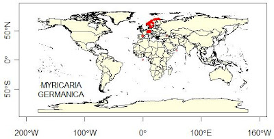
Nice Species Distribution Maps with GBIF-Data in R

Here's an example of how to easily produce real nice distribution maps from GBIF-data in R with package maps...

Use of Classification Trees to Investigate Traits of Invasive Species

Which traits make an alien species invasive?
Due to what traits an alien species becomes established in a foreign flora?


This kind of questions could be analysed by the use of recursive partitioning and classification trees..
(the below example also includes some useful data manipulation techniques)...

Comparing Two Distributions

Here I compare two distributions, flowering duration of indigenous and allochtonous plant species. The hypothesis is that alien compared to indigenous plant species exhibit longer flowering periods.

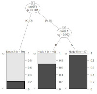
Test Difference between Two Proportions & Plot Confidence Intervals

..an illustrative example for testing proportions and presenting the results.

the data: number of indigenous and alien plant species with and without vegetative reproduction (N = 3399, mid-european species, data-courtesy: BiolFlor) . Hypothesis: The proportion of species with vegetative reproduction is different between alien and indigenuos plant species.

result:  the prop. of plants with veg. reproduction is sign. lower for alien compared to indigenous plant species. this is simply due to the large number of agricultural weeds and contaminants within alien species - these species almost always reproduce by seeds.

## data:
dat <- data.frame(list(structure(list(flstat = structure(c(2L, 1L, 2L, 1L),
.Label = c("allo", "auto"), class = "factor"),
reprod = structure(c(1L, 1L, 2L, 2L),
.Label = c("non-veg", "veg"), class = "factor"),
X = c(872L, 423L, 1872L, 232L)),
.Names = c("flstat", "reprod", "X"),
class = "data.frame", row.names = c(NA, -4L))))

## proportion of species with vegetative reproduction
p_allo <- dat$X[4] / (dat$X[2] + dat$X[4])
p_auto <- dat$X[3] / (dat$X[1] + dat$X[3])
p_allo
p_auto

## restructure data for glm:
dat1 <- dat[rep(1:4, dat$X), 1:2]
head(dat1)
dat1$inc <- ifelse(dat1$reprod == "non-veg", 0, 1)

## glm:
summary(gmod <- glm(inc ~ flstat, data = dat1, family = binomial))

## intercept = logit(p_allo):
print(est_p_allo <- plogis(gmod$coef[1]))

## intercept + b = logit(p_allo+p_auto):
print(est_p_auto <- plogis(gmod$coef[1] + gmod$coef[2]))

## alternatively test difference in two proportions with prop.test():
ptest_diff <- prop.test(x = c(dat$X[1], dat$X[2]),
                        n = c(dat$X[1] + dat$X[3], dat$X[2] + dat$X[4]))

## only for one proportion prop.test gives you the confidence
## intervals of p.
## (you could also extract the glm-standard errors and calculate
## the conf.int. for this purpose..):
ptest_auto <- prop.test(x = dat$X[3], n = dat$X[1] + dat$X[3])
ptest_allo <- prop.test(x = dat$X[4], n = dat$X[2] + dat$X[4])

## plot with confidence intervals from prop.test
## (see methods in ?prop.test):

## coordinates for plotting confidence interval bars:
y0_al <- ptest_allo$conf[1]
y1_al <- ptest_allo$conf[2]
y0_au <- ptest_auto$conf[1]
y1_au <- ptest_auto$conf[2]

library(grid)
library(lattice)

## panel function for suppressing tck at top and right side,
## drawing bar with confidence interval,
## plotting glm-estimates (the crosses)
mpanel = function(...) {grid.segments(x0 = c(0.2725, 1 - 0.2725),
                                      x1 = c(0.2725, 1 - 0.2725),
                                      y0 = c(y0_al, y0_au),
                                      y1 = c(y1_al, y1_au))
                        panel.points(x = c(0.8, 2.2),
                                    y = c(est_p_allo, est_p_auto), pch = 4)
                        panel.abline(h = c(p_allo, p_auto), lty = 15,
                                     col = "grey70")
                        panel.text(x = 1.5, y = 0.9, cex = 1.2,
                                   "Species With\nVegetative Reproduction");
                        panel.xyplot(...)}

xyplot(c(p_allo, p_auto) ~ as.factor(c("Alien", "Indigenous")), type = "b",
       ylab = "Prop. +/- CIs\nX = GLM-Estimates",
       xlab = "", ylim = c(0, 1),
       panel = mpanel, pch = 16,
       scales = list(alternating = 1, tck = c(1, 0)))

Two-Way PERMANOVA (adonis, vegan-Package) with Customized Contrasts

...say you have a multivariate dataset and a two-way factorial design - you do a PERMANOVA and the aov-table (adonis is using ANOVA or "sum"-contrasts) tells you there is an interaction - how to proceed when you want to go deeper into the analysis?
You could, however somewhat tedious, customize contrasts for the PERMANOVA and check for differences between certain level combinations.

Multiple Comparisons for GLMMs using glmer() & glht()

...here's an example of how to apply multiple comparisons to a generalised linear mixed model (GLMM) using the function glmer from package lme4 & glht() from package multcomp. Also, I present a nice example for visualizing data from a nested sampling design with lattice-plots! 

How to List all Functions of an R-Package

ls("package:base")
   [1] "-"                                  "-.Date"                            
   [3] "-.POSIXt"                           "!"                                 
   [5] "!.hexmode"                          "!.octmode"                         
   [7] "!="                                 "$"                                 
   [9] "$.DLLInfo"                          "$.package_version"                 
  [11] "$<-"                                "$<-.data.frame"                    
  [13] "%%"                                 "%*%"                               
  [15] "%/%"                                "%in%"                              
  [17] "%o%"                                "%x%"                               
  [19] "&"                                  "&&"                                
  [21] "&.hexmode"                          "&.octmode"                         
  [23] "("                                  "*"    
...

lsf.str("package:base")
- : function (e1, e2)  
-.Date : function (e1, e2)  
-.POSIXt : function (e1, e2)  
! : function (x)  
!.hexmode : function (a)  
!.octmode : function (a)  
!= : function (e1, e2)  
$ : .Primitive("$") 
...

Drawing Grids in R

Here's an example of how to draw a grid in R and how to fill it.
I did use the grid-package and its functions for displaying species cover values at squares of a recording frame...

Legendre & Borcard: Nested ANOVA by Permutation

..here's a very illustrative R-Script example by Legendre & Borcard showing how a Nested ANOVA can be done by permutation.

Summarize Data by Several Variables

Here's an example how to conveniently summarize data with the cast function (package reshape). By the way you see how this could be done "in-conveniently" by hand. You also see how a for-loop works and how a matrix is constructed and filled. In addition this serves as an illustrative example how flexible "indexing" in R works, as seen in the below loop! (download data) (this example is adapted from https://stat.ethz.ch/pipermail/r-sig-ecology/2011-May/002174.html)

Fit Sigmoid Curve with Confidence Intervals

Sigmoid curve fitting for transpiration measurements from porometer at different water potentials (pressure):

Adonis (PERMANOVA) - Assumptions

Before you use PERMANOVA (R-vegan function adonis) you should read the user notes for the original program by the author (Marti J. Anderson) who first came up with this method. An important assumtption for PERMANOVA is same "multivariate spread" among groups, which is similar to variance homogeneity in univariate ANOVA.

I'll show why you may draw the wrong conclusions if this assumption is not met:

Permutation Test with Stratified Data and Repeated Measurements

This is an example for a permutation test on stratified samples with repeated measurements. Samples are interdependent firstly because they come from several sites and secondly because the sampling was repeated a second time. That is samples of the same sites are dependent and sample t1 and sample t2, taken from the very same places are dependent. 

What I want to test is whether there is a difference between timepoint one (t1) and two (t2) or not. A hypothesis could be: the average difference t1-t2 is sign. larger than zero (a one-sided test). Another hypothesis could be: the average difference is sign. different from zero, either larger or smaller (a two-sided test).

If you deal with a distribution of your data that ordinary Linear Mixed Models (LMMs) or Generalized LMMs (GLMMs) can handle you should vote for this option - but sometimes you deal with awkard data and permutation tests may the only thing to bail you out...

Bootsrap Confidence Intervals, Stratified Bootstrap

 Here's a worked example for comparing group averages with bootstrap confidence intervals and allowing for different subsample sizes by calling the strata argument within the bootstrap function.

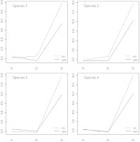
The data (simulated) is set up analogous to an before-after impact experiment conducted on plots across 4 levels of a grouping factor ('stage'). Similarities were calculated for each composition before and after an impact and will be averaged over the grouping factor. Our hypothesis was that the levels of the grouping factor would show significantly different average similarities - that is, a higher/lower impact on composition. As plots were aggregated in different sites within the 'stages', this dependency had to be allowed for by use of the "strata" argument in the boot.ci call.

The conclusion from this simulated example would be that the averages similarities at stages C and D are significantly different from stages A and B. That is, as the similarities are higher in C and D than in A and B, impact on composition is significantly lower in C and D.

Custom Labels for Ordination Diagram

Here is how you do custom labels, hull, spider in a vegan ordination diagram:

Test Difference Between Diversity-Indices of Two Samples with Abundance Data

I adapted a permutation test from the PAST Software (Hammer & Harper, http://folk.uio.no/ohammer/past/diversity.html) that tests difference between diversity-indices of two samples with abundance data in R... See the example below:

Multivariate Repeated Measurements with adonis():

Please check the updated code in the comment by Wallace Beiroz, 26 January 2015 at 13:37!

Lately I had to figure out how to do a repeated measures (or mixed effects) analysis on multivariate (species) data. Here I share code for a computation in R with the adonis function of the vegan package. Credit goes to Gavin Simpson providing most of the important pieces of the below code in R-Help.