Duplicate a figure with R

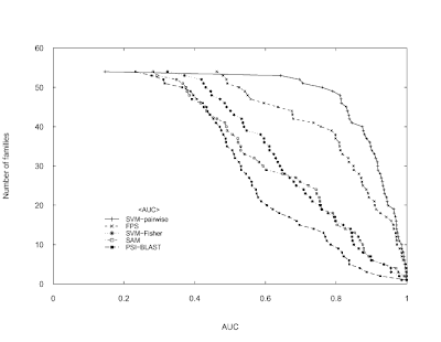
The following code attempts to reproduce the Figure 3 (top) in Liao L, Noble WS.
Combining pairwise sequence similarity and support vector machines for detecting remote protein evolutionary and structural relationships. Journal of computational biology. 2003;10(6):857-68 using only the Base graphics system in R.
Data can be downloaded from here (if it doesn't work, use Google's cache).
I imported the file in a spreadsheet and then I copied & pasted it in R.

jcb.scores = read.delim("clipboard")
attach(jcb.scores)
pdf("recomb_scores.pdf")
par(las =1) # To have horizontal labels for axes 2 and 4
plot(y~sort(SVM.pairwise.ROC, decreasing = TRUE), pch = 3, cex = 0.5,
xlab = "AUC", ylab = "Number of families", axes = FALSE,
xlim = c(0,1), ylim = c(0,60))
lines(y~sort(SVM.pairwise.ROC, decreasing = TRUE), lty = 1)
points(y~sort(FPS.ROC, decreasing = TRUE), pch = 4, cex = 0.5)
lines(y~sort(FPS.ROC, decreasing = TRUE), lty = 2)
points(y~sort(SVM.Fisher.ROC, decreasing = TRUE), pch = 8, cex = 0.5)
lines(y~sort(SVM.Fisher.ROC, decreasing = TRUE), lty = 3)
points(y~sort(SAM.ROC, decreasing = TRUE), pch = 0, cex = 0.5)
lines(y~sort(SAM.ROC, decreasing = TRUE), lty = 4)
points(y~sort(PSI.BLAST.ROC, decreasing = TRUE), pch = 15, cex = 0.5)
lines(y~sort(PSI.BLAST.ROC, decreasing = TRUE), lty = 5)
axis(1, at = seq(0,1,0.2), labels = c(0,0.2,0.4,0.6,0.8,1), tcl = 0.25, pos = 0) # tcl = 0.25 small ticks toward the curve
axis(2, at = c(0,10,20,30,40,50,60), labels=c(0,10,20,30,40,50,60), tcl= 0.25 , pos = 0)
axis(2, at = c(0,10,20,30,40,60), tcl= 0.25,labels = F, pos = 0)
axis(3, tick = T, tcl= 0.25, labels = F, pos = 60)
axis(4, at = c(0,10,20,30,40,50), tcl= 0.25, labels = F, pos = 1)
axis(4, at = c(0,10,20,30,40,60), tcl= 0.25, labels = F, pos = 1)
# To locate the legend interactively
xy.legend = locator(1)
# right-justifying a set of labels: thanks to Uwe Ligges
temp <- legend(xy.legend, legend = c("SVM-pairwise", "FPS","SVM-Fisher", "SAM","PSI-BLAST"), text.width = strwidth("SVM-pairwise"), xjust = 1, yjust = 1, lty = c(1,2,3,4,5), pch = c(3,4,8,0,15), bty = "n", cex = 0.8, title = "")
dev.off()
detach(jcb.scores)

The original image:

My version of the image (not exacly identical but...):

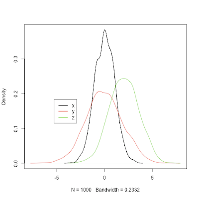
Plotting two or more overlapping density plots on the same graph

This post was updated.
See this thread from StackOverflow for other ways to solve this task.

plot.multi.dens <- function(s)
{
junk.x = NULL
junk.y = NULL
for(i in 1:length(s))
{
junk.x = c(junk.x, density(s[[i]])$x)
junk.y = c(junk.y, density(s[[i]])$y)
}
xr <- range(junk.x)
yr <- range(junk.y)
plot(density(s[[1]]), xlim = xr, ylim = yr, main = "")
for(i in 1:length(s))
{
lines(density(s[[i]]), xlim = xr, ylim = yr, col = i)
}
}
#usage:
x = rnorm(1000,0,1)
y = rnorm(1000,0,2)
z = rnorm(1000,2,1.5)
# the input of the following function MUST be a numeric list
plot.multi.dens(list(x,y,z))
library(Hmisc)
le <- largest.empty(x,y,.1,.1)
legend(le,legend=c("x","y","z"), col=(1:3), lwd=2, lty = 1)

R package installation and administration

A short list of basic but useful commands for managing
the packages in R:

# install a package
install.packages("ROCR")
# visualize package version
package_version("pamr")
# update a package
update.packages("Cairo")
# remove a package
remove.packages("RGtk2")

Sorting/ordering a data.frame according specific columns


x = rnorm(20)
y = sample(rep(1:2, each = 10))
z = sample(rep(1:4, 5))

data.df <- data.frame(values = x, labels.1 = y, labels.2 = z)
print(data.df)

# data ordered according to "labels.1" column
# and then "labels.2" column
nams <- c("labels.1", "labels.2")
data.df.sorted = data.df[do.call(order, data.df[nams]), ]
print(data.df.sorted)


Receiver Operating Characteristic (ROC) Curve in ROCR and verification packages

The following VERY basic code shows how to plot a simple ROC Curve both by means of ROCR package and by verification package.

# it allows two different plots in the same frame
par(mfrow = c(1,2))
# plot a ROC curve for a single prediction run
# and color the curve according to cutoff.
library(ROCR)
data(ROCR.simple)
pred <- prediction(ROCR.simple$predictions, ROCR.simple$labels)
perf <- performance(pred,"tpr", "fpr")
plot(perf,colorize = TRUE)
# plot a ROC curve for a single prediction run
# with CI by bootstrapping and fitted curve
library(verification)
roc.plot(ROCR.simple$labels,ROCR.simple$predictions, xlab = "False positive rate",
ylab = "True positive rate", main = NULL, CI = T, n.boot = 100, plot = "both", binormal = TRUE)

screen - an other VERY useful Unix tool

from R News Vol. 7/1 April 2007 (http://cran.r-project.org/doc/Rnews/Rnews_2007-1.pdf):
If you need to run R code that executes for long periods of time upon remote machines, this amazing unix tool would became your best friend!
screen is a so-called terminal multiplexor, which allows us to create, shuffle, share, and suspend command line sessions within one window. It provides protection against disconnections and the flexibility to retrieve command line sessions remotely.

Starting using this utility is easy like ABC:

1. Log in to remote server
2. Run screen
3. Run R and the long calculation
4. Detach screen (Ctrl-a, Ctrl-d)
5. Logout

The R session continues working in the background, contained within the screen session. If we want to revisit the session to check its progress, then we:

1. Log in remotely via secure shell
2. Start screen -r, which recalls the unattached session
3. Examine how your calculation/script is performing
4. Detach the screen session, (Ctrl-a, Ctrl-d)
5. Log out

This procedure can be used, clearly, for invoking whatever unix program/command you need to use; it is sufficient to substitute the R invoking command with your invoking command line program(for example python).

As usual in the shell-space, invoking man (man screen in this case) will provide all sort of information you need to know about the tool.

R upgrading on Windows© revisited

From the list:
When I update R the following has worked for me (Windows XP)
1. Install the new version to a new directory (say C:\Program Files\R\R-2.5.1).
2. Rename the new library subdirectory to library2.
3. Copy the entire contents of the old library subdirectory (say
C:\Program Files\R\R-2.4.0\library\ to the new R root to create
C:\Program Files\R\R-2.5.1\library\ .
4. Copy the contents of library2 to library to update your basic library.
5. Now start your new version of R and update packages from the GUI or
from the R console. (You may need to firs check Rprofile .site to
ensure that no packages have been loaded)
6. On occasion I have got warning messages when I tried to load
packages after this procedure. This has been cleared by running
update.packages(checkBuilt = TRUE)
This checks that your packages have been built with the latest
version. When I do this I agree to install all available updates.
7. You may wish to copy various autoloads etc from your old
Rprofile.site to your new Rprofile.site. I understand that there are
some compatibility problems with 2.5.1 and SciViews so be careful.