Classification: a quick and dirty example

## Thanks to the UCI repository Magic Gamma telescope data set
magic04 = read.table("http://archive.ics.uci.edu/ml/machine-learning-databases/magic/magic04.data", header = F, sep=",")
# split the data set in test and training set
split.data <- function(data, p = 0.7, s = 666){
set.seed(s)
index <- sample(1:dim(data)[1])
train <- data[index[1:floor(dim(data)[1] * p)], ]
test <- data[index[((ceiling(dim(data)[1] * p)) + 1):dim(data)[1]], ]
return(list(train = train, test = test))
}
dati = split.data(magic04, p = 0.7)
train = dati$train
test = dati$test
# SVM training just for fun
library(e1071)
model <- svm(train[,1:10],train[,11], probability = T)
# prediction on the test set
pred <- predict(model, test[,1:(dim(test)[[2]]-1)], probability = T)
# Check the predictions
table(pred,test[,dim(test)[2]])
pred.prob <- attr(pred, "probabilities")
pred.to.roc <- pred.prob[, 1]
# performance assessment
library(ROCR)
pred.rocr <- prediction(pred.to.roc, as.factor(test[,(dim(test)[[2]])]))
perf.rocr <- performance(pred.rocr, measure = "auc", x.measure = "cutoff")
cat("AUC =",deparse(as.numeric(perf.rocr@y.values)),"\n")
perf.tpr.rocr <- performance(pred.rocr, "tpr","fpr")
plot(perf.tpr.rocr, colorize=T)

Hello World for Clustering methods

A hello world program can be a useful sanity test to make sure that the procedure/methods you are analyzing "works" at least for very basic tasks. For this purpose, I create an artificial data set from 4 different 2-dimensional normal distributions to check how well the 4 clusters can be recognized by common clustering methods.

set1 <- matrix(cbind(rnorm(100,0,2),rnorm(100,0,2)),100,2)
set2 <- matrix(cbind(rnorm(100,0,2),rnorm(100,8,2)),100,2)
set3 <- matrix(cbind(rnorm(100,8,2),rnorm(100,0,2)),100,2)
set4 <- matrix(cbind(rnorm(100,8,2),rnorm(100,8,2)),100,2)
dati <- list(values=rbind(set1,set2,set3,set4),classes=c(rep(1,100),rep(2,100),rep(3,100),rep(4,100))) # clustering - common methods
op <- par(mfcol = c(2, 2))
par(las =1)
plot(dati$values, col = as.integer(dati$classes), xlim=c(-6,14), ylim = c(-6,14), xlab="", ylab="", main = "True Groups")
party <- kmeans(dati$values,4)
plot(dati$values, col = party$cluster, xlab = "", ylab = "", main = "kmeans")
hc = hclust(dist(dati$values), method = "ward")
memb <- cutree(hc, k = 4)
plot(dati$values, col = memb, xlab = "", ylab = "", main = "hclust Euclidean ward") hc = hclust(dist(dati$values), method = "complete")
memb <- cutree(hc, k = 4)
plot(dati$values, col = memb, xlab = "", ylab = "", main = "hclust Euclidean complete")
par(op)



This is one of that tiny function that help you to save yourself a lot of time! I thank the list for the suggestion!

library(gdata)
?keep
data(women, cars)
keep(cars)
## To remove all objects except cars, run:
## keep(cars, sure=TRUE)


Duplicate a figure with R

The following code attempts to reproduce the Figure 3 (top) in Liao L, Noble WS.
Combining pairwise sequence similarity and support vector machines for detecting remote protein evolutionary and structural relationships. Journal of computational biology. 2003;10(6):857-68 using only the Base graphics system in R.
Data can be downloaded from here (if it doesn't work, use Google's cache).
I imported the file in a spreadsheet and then I copied & pasted it in R.

jcb.scores = read.delim("clipboard")
attach(jcb.scores)
pdf("recomb_scores.pdf")
par(las =1) # To have horizontal labels for axes 2 and 4
plot(y~sort(SVM.pairwise.ROC, decreasing = TRUE), pch = 3, cex = 0.5,
xlab = "AUC", ylab = "Number of families", axes = FALSE,
xlim = c(0,1), ylim = c(0,60))
lines(y~sort(SVM.pairwise.ROC, decreasing = TRUE), lty = 1)
points(y~sort(FPS.ROC, decreasing = TRUE), pch = 4, cex = 0.5)
lines(y~sort(FPS.ROC, decreasing = TRUE), lty = 2)
points(y~sort(SVM.Fisher.ROC, decreasing = TRUE), pch = 8, cex = 0.5)
lines(y~sort(SVM.Fisher.ROC, decreasing = TRUE), lty = 3)
points(y~sort(SAM.ROC, decreasing = TRUE), pch = 0, cex = 0.5)
lines(y~sort(SAM.ROC, decreasing = TRUE), lty = 4)
points(y~sort(PSI.BLAST.ROC, decreasing = TRUE), pch = 15, cex = 0.5)
lines(y~sort(PSI.BLAST.ROC, decreasing = TRUE), lty = 5)
axis(1, at = seq(0,1,0.2), labels = c(0,0.2,0.4,0.6,0.8,1), tcl = 0.25, pos = 0) # tcl = 0.25 small ticks toward the curve
axis(2, at = c(0,10,20,30,40,50,60), labels=c(0,10,20,30,40,50,60), tcl= 0.25 , pos = 0)
axis(2, at = c(0,10,20,30,40,60), tcl= 0.25,labels = F, pos = 0)
axis(3, tick = T, tcl= 0.25, labels = F, pos = 60)
axis(4, at = c(0,10,20,30,40,50), tcl= 0.25, labels = F, pos = 1)
axis(4, at = c(0,10,20,30,40,60), tcl= 0.25, labels = F, pos = 1)
# To locate the legend interactively
xy.legend = locator(1)
# right-justifying a set of labels: thanks to Uwe Ligges
temp <- legend(xy.legend, legend = c("SVM-pairwise", "FPS","SVM-Fisher", "SAM","PSI-BLAST"), text.width = strwidth("SVM-pairwise"), xjust = 1, yjust = 1, lty = c(1,2,3,4,5), pch = c(3,4,8,0,15), bty = "n", cex = 0.8, title = "")
dev.off()
detach(jcb.scores)

The original image:

My version of the image (not exacly identical but...):

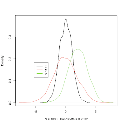
Plotting two or more overlapping density plots on the same graph

This post was updated.
See this thread from StackOverflow for other ways to solve this task.

plot.multi.dens <- function(s)
{
junk.x = NULL
junk.y = NULL
for(i in 1:length(s))
{
junk.x = c(junk.x, density(s[[i]])$x)
junk.y = c(junk.y, density(s[[i]])$y)
}
xr <- range(junk.x)
yr <- range(junk.y)
plot(density(s[[1]]), xlim = xr, ylim = yr, main = "")
for(i in 1:length(s))
{
lines(density(s[[i]]), xlim = xr, ylim = yr, col = i)
}
}
#usage:
x = rnorm(1000,0,1)
y = rnorm(1000,0,2)
z = rnorm(1000,2,1.5)
# the input of the following function MUST be a numeric list
plot.multi.dens(list(x,y,z))
library(Hmisc)
le <- largest.empty(x,y,.1,.1)
legend(le,legend=c("x","y","z"), col=(1:3), lwd=2, lty = 1)

R package installation and administration

A short list of basic but useful commands for managing
the packages in R:

# install a package
install.packages("ROCR")
# visualize package version
package_version("pamr")
# update a package
update.packages("Cairo")
# remove a package
remove.packages("RGtk2")

Sorting/ordering a data.frame according specific columns


x = rnorm(20)
y = sample(rep(1:2, each = 10))
z = sample(rep(1:4, 5))

data.df <- data.frame(values = x, labels.1 = y, labels.2 = z)
print(data.df)

# data ordered according to "labels.1" column
# and then "labels.2" column
nams <- c("labels.1", "labels.2")
data.df.sorted = data.df[do.call(order, data.df[nams]), ]
print(data.df.sorted)