R 2.11.0 is released!

The new R 2.11.0 is out! Get it from here.
Take a look at these posts for some miscellaneous advices to make the upgrade easier.
Also this thread on stackoverflow can be of some value.
Feel free to contribute with suggestions about how to upgrade your R installation.

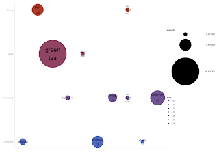
Balloon plot using ggplot2

Following Tal Galili example and using part of his code, I want to plot the balloonplot you can see here using R and the excellent ggplot2 package by Hadley Wickham.

### I retrieve the data from the google document you can find here using Tal Galili code:
## I slightly modified Tal code to include popularity stats:
supplement.popularity <- supplements.data[ss,7]
supplements.df <- na.omit(data.frame(supplement.name, supplement.benefits, supplement.popularity, supplement.score)) ## remove rows containing NAs
colnames(supplements.df) <- c("name", "benefits", "popularity", "score")
## For sake of simplicity I select only the cardio metacondition
cardio <- (supplements.df[supplement.benefits=="cardio",])[, -2]

## For reproducibility I add the cardio data.frame so you can use it right away
cardio <- read.table(tc <-textConnection(
" name popularity score
2 'arginine' 1.080 3
10 'vitamin b3' 0.201 3
15 'omega 3' 4.000 3
22 'hawthorn' 0.442 4
27 'red yeast rice' 0.264 4
29 'vitamin d' 6.700 4
31 'omega 6' 2.000 4
35 'green tea' 26.100 5
37 'olive leaf' 0.224 5
41 'fish oil' 4.000 6
43 'red yeast rice' 0.264 6")); close(tc)
cardio$name <- gsub(" ", "\n", cardio$name) #substitute ' ' with '\n' in the names

library(ggplot2)
myTheme <- function(base_size = 10) {
structure(list(
panel.background = theme_rect(size = 1, colour = "lightgray"),
panel.grid.major = theme_blank(),
panel.grid.minor = theme_blank(),
axis.line = theme_blank(),
axis.text.x = theme_blank(),
axis.ticks = theme_blank(),
strip.background = theme_blank(),
strip.text.y = theme_blank(),
legend.background = theme_blank(),
legend.key = theme_blank(),
legend.key.size = unit(1.2, "lines"),
legend.title = theme_text(size = 8, face = "bold", hjust = 0),
legend.position = "right"
), class = "options")
}

s <- ggplot(cardio, aes(name, score)) + xlab(NULL) + ylab(NULL) + myTheme()
s <- s + geom_point( aes(size=popularity, colour=score, fill=score), legend=TRUE) +
scale_y_continuous( breaks=as.numeric(levels(factor(cardio$score))), labels=c("Conflicting", "Promising", "Good", "Strong") ) +
scale_area( breaks=c(min(cardio$popularity),mean(cardio$popularity),max(cardio$popularity)), to=c(4,60) ) +
geom_text(aes(y=cardio$score, label=cardio$name, size=cardio$popularity/90), legend=FALSE)
#pdf("cardio.pdf",height=8,width=12);s;dev.off()
png("cardio.png",height=700,width=1000);s;dev.off()

One R Tip A Day meets Tecnica Arcana

For italian speaking people only (sorry!).

Carlo il curatore dell'ottimo podcast tecnologico Tecnica Arcana mi ha intervistato sulla mia professione e su R. Qui potete scaricare l'intervista in formato mp3.

Scatter plot with 4 axes labels and grid

Ravi from this post (via Revolutions blog) wanted to check the code that produces the left panel of the Figure 3 from this article taken from the current issue of the R Journal. Below my attempt to reproduce the plot:

rv <- seq(1.3, 2.9, .1)
rv <- rv[-grep("1.6", rv)] # remove R version 1.6
pckg.num <- c(110,129,162,219,273,357,406,548,647,739,911,1000,1300,1427,1614,1952)
rv.dates <- c("2001-6-21", "2001-12-17","2002-06-12","2003-05-27",
"2003-11-16","2004-06-05","2004-10-12","2005-06-18","2005-12-16", "2006-05-31",
"2006-12-12","2007-04-12","2007-11-16","2008-03-18","2008-10-18","2009-09-17")
pckg.fit <- lm(pckg.num~rv)
png("CRAN_packages.png")
par(mar=c(7, 5, 5, 3), las=2)
plot(as.POSIXct(rv.dates), pckg.num, xlab="",ylab="",col="red", log="y", pch=19, axes=F)
axis.POSIXct(1, 1:16, rv.dates, format="%Y-%m-%d")
mtext("Date", side=1, line=5, las=1)
axis(2, at=c(100,200,300,400,500,600,800,100,1200,1500,2000))
mtext("Number of CRAN Packages", side=2, line=3, las=3)
axis.POSIXct(3, rv.dates, rv.dates, labels=as.character(rv))
mtext("R Version", side=3, line=3, las=1)
axis(4, pckg.num)
abline(v=as.POSIXct(rv.dates), col="lightgray", lty="dashed")
abline(h=pckg.num, col="lightgray", lty="dashed")
box()
abline(lm(log10(pckg.num)~as.POSIXct(rv.dates)), col="red")
dev.off()


R Journal 1/2

R Journal 1/2 is out! Grab it from here.

A central hub for R bloggers

I would like to suggest to my readers to take a look and bookmark a new blog named R-bloggers which aims to be "a central hub of content collected from bloggers who write about R".
It seems a nice idea to me to have a centralized source of information for the R blogger community.
Good Luck, Tal!

R in Action - early thoughts

I was invited to review the book R in Action written by Rob Kabacoff. Since I consider the Quick-R website, created by the same smart guy, one of the most valuable resources about R, It is both an honor and a pleasure to have the opportunity to take an early look at his book and to express some thoughts about it.

First, this book is distributed under an early access policy that means, as it is stated on the editor's web site, that: This Early Access version of the book enables you to receive new chapters as they are being written. You can also interact with the authors to ask questions, provide feedback and errata, and help shape the final manuscript on the Author Online. This is a nice publishing approach, the editor settled up an ad-hoc forum which allows real-time feedback from early adopters. This beta-test sort of approach is convenient both to the author that can fix errata and improve contents before the final version is published and to the early adopters that can access to useful contents in advance and receive valuable explanations directly from the author.

Since only the initial part of the book is available, this short review will be at most incomplete and present only preliminary thoughts. I'm going to update the review as soon as I have the possibility to read the rest of the book.

R in Action, as mimicked in its structure, aims to guide the new adopters from the vary basics of the language through to the most advanced features by a progressive task-driven approach carefully curated by the author.

In the initial part of the book, Kabacoff covers all the basic features of the language from data manipulation to the basic statistics required to make sense of the data plus the most common and useful graphical methods for visualizing them.

The author makes large use of working example. This is one of the most effective teaching technique, in my opinion, because it encourages readers to apply immediately the knowledge acquired.

An other nice ingredient of Kabacoff method is to introduce effective high quality packages from the huge R collection to solve a proposed task. For example, in chapter three the author introduces the rename function from the awesome reshape package to rename the columns of a data.frame. This is a very trivial task, that can be easily managed by standard R (as the author shows shortly afterward); but the smoothly introduction of this useful package, explained and used more extensively in the forthcoming chapters, represents a nice touch that both means to manage the task in a more elegant way and introduces the user to a powerful tool.
In this fashion, the tasks presented in the text are addressed using several different packages in order to depict the various alternative methods available in R.
Furthermore, the numerous notes accompanying the explanations serve both to make easier the understanding of the described concepts and to provide useful insights about R features and idiosyncrasies.

To sum up, the chapters I had the opportunity to examine are a solid base for people getting started with R. I'm impatient to dig through the forthcoming chapters of the book which deal with advanced statistics and graphics!

I warmly recommend this book even in this early stage: if you are new to R programming this is a valid approach to start being familiar with the language and make effective use of it in from day one.