R Journal 2/1

R Journal 2/1 is out! Grab it from here.

R 2.11.0 is released!

The new R 2.11.0 is out! Get it from here.
Take a look at these posts for some miscellaneous advices to make the upgrade easier.
Also this thread on stackoverflow can be of some value.
Feel free to contribute with suggestions about how to upgrade your R installation.

Balloon plot using ggplot2

Following Tal Galili example and using part of his code, I want to plot the balloonplot you can see here using R and the excellent ggplot2 package by Hadley Wickham.

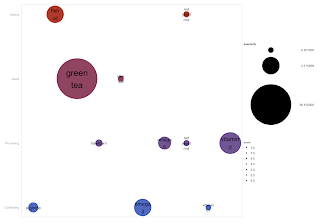
### I retrieve the data from the google document you can find here using Tal Galili code:
## I slightly modified Tal code to include popularity stats:
supplement.popularity <- supplements.data[ss,7]
supplements.df <- na.omit(data.frame(supplement.name, supplement.benefits, supplement.popularity, supplement.score)) ## remove rows containing NAs
colnames(supplements.df) <- c("name", "benefits", "popularity", "score")
## For sake of simplicity I select only the cardio metacondition
cardio <- (supplements.df[supplement.benefits=="cardio",])[, -2]

## For reproducibility I add the cardio data.frame so you can use it right away
cardio <- read.table(tc <-textConnection(
" name popularity score
2 'arginine' 1.080 3
10 'vitamin b3' 0.201 3
15 'omega 3' 4.000 3
22 'hawthorn' 0.442 4
27 'red yeast rice' 0.264 4
29 'vitamin d' 6.700 4
31 'omega 6' 2.000 4
35 'green tea' 26.100 5
37 'olive leaf' 0.224 5
41 'fish oil' 4.000 6
43 'red yeast rice' 0.264 6")); close(tc)
cardio$name <- gsub(" ", "\n", cardio$name) #substitute ' ' with '\n' in the names

library(ggplot2)
myTheme <- function(base_size = 10) {
structure(list(
panel.background = theme_rect(size = 1, colour = "lightgray"),
panel.grid.major = theme_blank(),
panel.grid.minor = theme_blank(),
axis.line = theme_blank(),
axis.text.x = theme_blank(),
axis.ticks = theme_blank(),
strip.background = theme_blank(),
strip.text.y = theme_blank(),
legend.background = theme_blank(),
legend.key = theme_blank(),
legend.key.size = unit(1.2, "lines"),
legend.title = theme_text(size = 8, face = "bold", hjust = 0),
legend.position = "right"
), class = "options")
}

s <- ggplot(cardio, aes(name, score)) + xlab(NULL) + ylab(NULL) + myTheme()
s <- s + geom_point( aes(size=popularity, colour=score, fill=score), legend=TRUE) +
scale_y_continuous( breaks=as.numeric(levels(factor(cardio$score))), labels=c("Conflicting", "Promising", "Good", "Strong") ) +
scale_area( breaks=c(min(cardio$popularity),mean(cardio$popularity),max(cardio$popularity)), to=c(4,60) ) +
geom_text(aes(y=cardio$score, label=cardio$name, size=cardio$popularity/90), legend=FALSE)
#pdf("cardio.pdf",height=8,width=12);s;dev.off()
png("cardio.png",height=700,width=1000);s;dev.off()

One R Tip A Day meets Tecnica Arcana

For italian speaking people only (sorry!).

Carlo il curatore dell'ottimo podcast tecnologico Tecnica Arcana mi ha intervistato sulla mia professione e su R. Qui potete scaricare l'intervista in formato mp3.

Scatter plot with 4 axes labels and grid

Ravi from this post (via Revolutions blog) wanted to check the code that produces the left panel of the Figure 3 from this article taken from the current issue of the R Journal. Below my attempt to reproduce the plot:

rv <- seq(1.3, 2.9, .1)
rv <- rv[-grep("1.6", rv)] # remove R version 1.6
pckg.num <- c(110,129,162,219,273,357,406,548,647,739,911,1000,1300,1427,1614,1952)
rv.dates <- c("2001-6-21", "2001-12-17","2002-06-12","2003-05-27",
"2003-11-16","2004-06-05","2004-10-12","2005-06-18","2005-12-16", "2006-05-31",
"2006-12-12","2007-04-12","2007-11-16","2008-03-18","2008-10-18","2009-09-17")
pckg.fit <- lm(pckg.num~rv)
png("CRAN_packages.png")
par(mar=c(7, 5, 5, 3), las=2)
plot(as.POSIXct(rv.dates), pckg.num, xlab="",ylab="",col="red", log="y", pch=19, axes=F)
axis.POSIXct(1, 1:16, rv.dates, format="%Y-%m-%d")
mtext("Date", side=1, line=5, las=1)
axis(2, at=c(100,200,300,400,500,600,800,100,1200,1500,2000))
mtext("Number of CRAN Packages", side=2, line=3, las=3)
axis.POSIXct(3, rv.dates, rv.dates, labels=as.character(rv))
mtext("R Version", side=3, line=3, las=1)
axis(4, pckg.num)
abline(v=as.POSIXct(rv.dates), col="lightgray", lty="dashed")
abline(h=pckg.num, col="lightgray", lty="dashed")
box()
abline(lm(log10(pckg.num)~as.POSIXct(rv.dates)), col="red")
dev.off()


R Journal 1/2

R Journal 1/2 is out! Grab it from here.

A central hub for R bloggers

I would like to suggest to my readers to take a look and bookmark a new blog named R-bloggers which aims to be "a central hub of content collected from bloggers who write about R".
It seems a nice idea to me to have a centralized source of information for the R blogger community.
Good Luck, Tal!